GetDP 
Patrick Dular and Christophe Geuzaine
GetDP is a general finite element solver that uses mixed finite elements to discretize de Rham-type complexes in one, two and three dimensions. This is the GetDP Reference Manual for GetDP 4.0.0 (development version) (May 16, 2026).
Table of Contents
- Obtaining GetDP
- Copying conditions
- Reporting a bug
- 1 Overview of GetDP
- 2 GetDP tutorial
- Further reading
- 2.1 Tutorial 1: Electrostatic field around a microstrip line
- 2.2 Tutorial 2: Thermal conduction in a radiator with fins
- 2.3 Tutorial 3: Magnetostatic model of an electromagnet
- 2.4 Tutorial 4: Magneto-quasistatic model of an electromagnet
- 2.5 Tutorial 5: Full-wave model of a rectangular waveguide
- 2.6 Tutorial 6: Global quantities in electrostatics
- 2.7 Tutorial 7: Magneto-thermal model of a three-phase busbar
- 2.8 Tutorial 8: Circuit coupling in 2D and 3D
- 2.9 Tutorial 9: Transformer model using a template library
- 2.10 Tutorial 9 bonus: Electromagnet model revisited using template library
- 2.11 Tutorial 10: Tree-cotree and Coulomb gauging
- 3 GetDP command-line interface
- 4 GetDP problem definition language
- 4.1 Expressions
- 4.2
Group: defining topological entities - 4.3
Function: defining global and piecewise expressions - 4.4
Constraint: specifying constraints on function spaces and formulations - 4.5
FunctionSpace: building function spaces - 4.6
Jacobian: defining jacobian methods - 4.7
Integration: defining integration methods - 4.8
Formulation: building equations - 4.9
Resolution: solving systems of equations - 4.10
PostProcessing: exploiting computational results - 4.11
PostOperation: exporting results - 4.12 Comments and includes
- 4.13 Macros, loops and conditionals
- Appendix A Internal file formats
- Appendix B Compiling the source code
- Appendix C Frequently asked questions
- Appendix D Version history
- Appendix E Copyright and credits
- Appendix F License
- Concept index
- Syntax index
Obtaining GetDP 
The source code and pre-compiled binary versions of GetDP (for Windows, macOS and Linux) can be downloaded from https://getdp.info. GetDP packages are also directly available in various Linux and BSD distributions (Debian, Fedora, Ubuntu, ...).
If you use GetDP, we would appreciate that you mention it in your work by citing the following paper: P. Dular, C. Geuzaine, F. Henrotte and W. Legros, A general environment for the treatment of discrete problems and its application to the finite element method. IEEE Transactions on Magnetics, 34(5), pp. 3395-3398, 1998.
Copying conditions 
GetDP is free software; this means that everyone is free to use it and to redistribute it on a free basis. GetDP is not in the public domain; it is copyrighted and there are restrictions on its distribution, but these restrictions are designed to permit everything that a good cooperating citizen would want to do. What is not allowed is to try to prevent others from further sharing any version of GetDP that they might get from you.
Specifically, we want to make sure that you have the right to give away copies of GetDP, that you receive source code or else can get it if you want it, that you can change GetDP or use pieces of GetDP in new free programs, and that you know you can do these things.
To make sure that everyone has such rights, we have to forbid you to deprive anyone else of these rights. For example, if you distribute copies of GetDP, you must give the recipients all the rights that you have. You must make sure that they, too, receive or can get the source code. And you must tell them their rights.
Also, for our own protection, we must make certain that everyone finds out that there is no warranty for GetDP. If GetDP is modified by someone else and passed on, we want their recipients to know that what they have is not what we distributed, so that any problems introduced by others will not reflect on our reputation.
The precise conditions of the license for GetDP are found in the General Public License that accompanies the source code (see License). Further information about this license is available from the GNU Project webpage http://www.gnu.org/copyleft/gpl-faq.html. Detailed copyright information can be found in Copyright and credits.
If you want to integrate parts of GetDP into a closed-source software, or want to sell a modified closed-source version of GetDP, you will need to obtain a different license. Please contact us directly for more information.
Reporting a bug 
If, after reading this reference manual, you think you have found a bug in GetDP, please file an issue on https://gitlab.onelab.info/getdp/getdp/issues. Provide as precise a description of the problem as you can, including sample input files that produce the bug. Don’t forget to mention both the version of GetDP and your operation system.
See Frequently asked questions, and the bug tracking system to see which problems we already know about.
1 Overview of GetDP 
GetDP is a finite element solver that uses conforming finite elements (nodal, edge, face and volume) to discretize de Rham complexes in one, two and three dimensions. Although originally designed for electromagnetic problems, it has grown into a general-purpose solver capable of handling a wide range of multiphysics problems, optionally coupled with lumped circuit elements. It supports 1D, 2D, 2D axisymmetric and 3D formulations, in steady-state, transient, time-harmonic and multi-harmonic regimes. Its defining feature is the close correspondence between the user-written ASCII description of a discrete problem and its symbolic mathematical formulation.
Over the last two decades, GetDP has been used to solve problems beyond the reach of other commercial or open-source finite element solvers: from nonlinear, strongly coupled h-phi magneto-quasistatic formulations with automatic cohomology basis functions on HPC clusters, to quasi-optimal, high-order non-overlapping Schwarz domain decomposition methods for high-frequency Helmholtz problems, to dynamic electrical machine simulations driven by neural-network-accelerated hysteresis models of ferromagnetic laminations.
GetDP’s modeling tools accommodate a broad spectrum of complexity, from quick demonstrations to advanced custom formulations, making the software well suited for research, education, training and industrial studies.
1.1 Numerical tools as objects 
In GetDP, a problem is defined by assembling computational tools (“objects”) into a structure that mirrors its mathematical formulation. This structure is written in a plain text data file (.pro file), so the equations describing a phenomenon serve directly as input to GetDP.
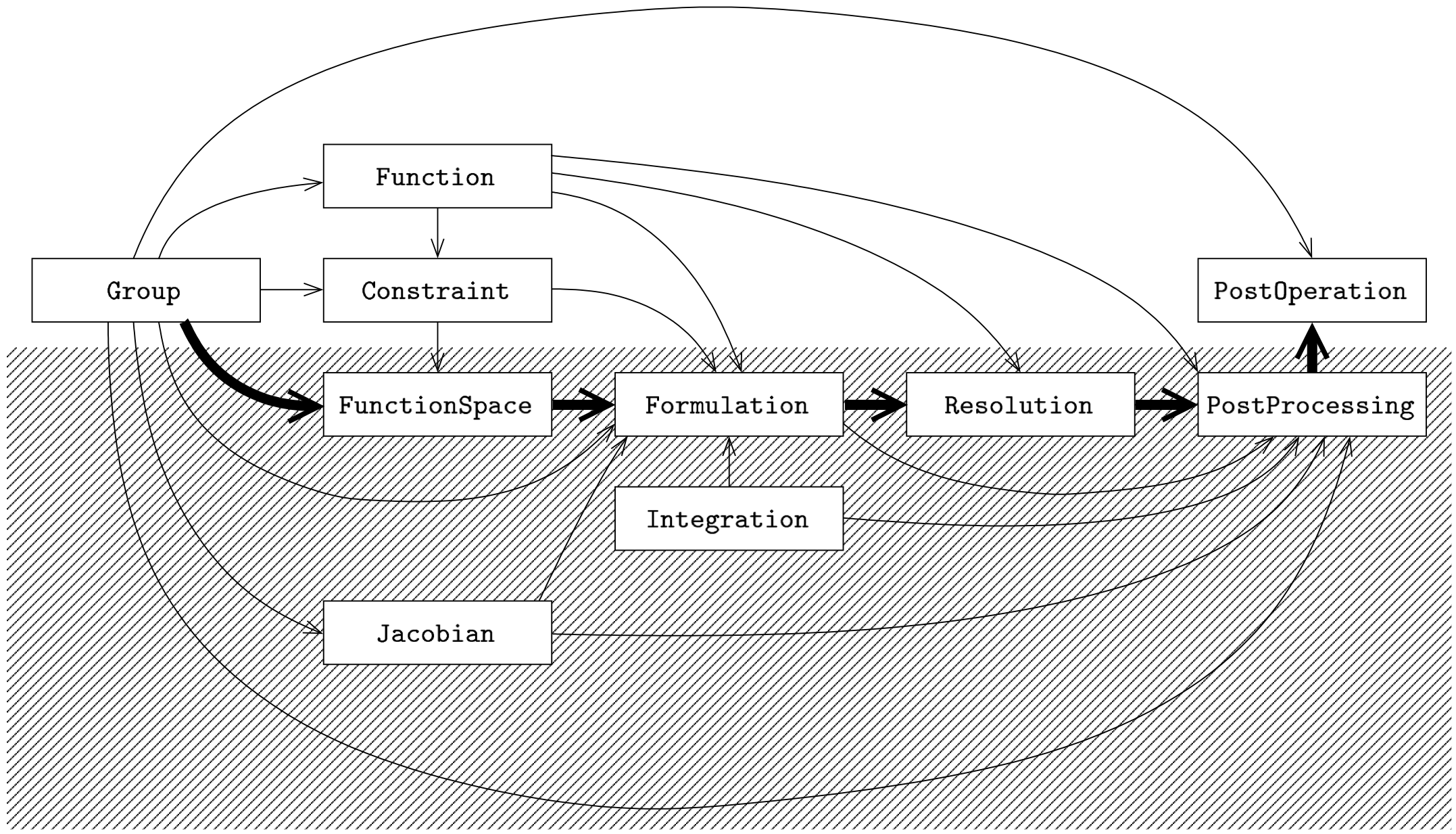
Solving a discrete problem with GetDP requires defining the ten objects listed below in a .pro file.
Object:         Depends on:
---------------------------------------------------------------
Group           ---
Function        Group
Constraint      Group, Function, (Resolution)
FunctionSpace   Group, Constraint, (Formulation), (Resolution)
Jacobian        Group
Integration     ---
Formulation     Group, Function, (Constraint), FunctionSpace,
                Jacobian, Integration
Resolution      Function, Formulation
PostProcessing  Group, Function, Jacobian, Integration,
                Formulation, Resolution
PostOperation   Group, PostProcessing
Reading the first column of the table above from top to bottom illustrates GetDP’s working philosophy and characteristic flow of operations, from group definitions to results visualization. The decomposition shown in the figure highlights the separation between the objects that define the solution method — which can be isolated into a “black box” (or “template”) (bottom) — and those that define the data specific to a given problem (top).
At the heart of every problem definition structure lie the formulations
(Formulation) and the function spaces
(FunctionSpace). Formulations define the systems of equations to
be assembled and solved; function spaces collect the quantities involved
in those formulations — functions, vector and covector fields, whether
known or unknown.
Each object in a problem definition structure must be defined before
being referenced by another. An ordering that always respects this
dependency is the following: first come the objects describing
problem-specific data — geometry, physical properties and boundary
conditions (Group, Function, Constraint) — then
those describing the solution method, such as unknowns, equations and
related objects (Jacobian, Integration,
FunctionSpace, Formulation, Resolution,
PostProcessing). The cycle ends with the presentation of the
results, defined in PostOperation objects, which produce outputs
in various formats. This decomposition makes it possible to build
templates that bundle the objects of the second group and apply to broad
classes of problems sharing a common solution method.
1.2 Bug reports 
Please file issues on https://gitlab.onelab.info/getdp/getdp/issues. Provide as precise a description of the problem as you can, including sample input files that produce the bug. Don’t forget to mention both the version of GetDP and the version of your operation system.
See Frequently asked questions, and the bug tracking system to see which problems we already know about.
2 GetDP tutorial 
The following tutorials provide a progressive introduction to GetDP. Each tutorial builds on the previous ones, introducing new modeling concepts, formulation techniques and solver features. They are designed to be studied in order.
- Electrostatics: Scalar potential formulation, Lagrange elements, Dirichlet boundary conditions.
- Thermal: Heat equation with conduction and convection, Neumann and Robin boundary conditions, steady-state and transient analyses, periodic constraints.
- Magnetostatics: Vector potential formulation, infinite elements, nonlinear materials with Newton-Raphson and Picard iterations.
- Magneto-quasistatics: Eddy currents, frequency- and time-domain analyses, axisymmetric models.
- Full wave: Edge elements, absorbing boundary conditions, Dirichlet constraint through an auxiliary resolution.
- Global quantities: Global basis functions, floating potentials, electrode charges and capacitances.
- Coupled problems: a-v formulation with global currents and voltages, magneto-thermal coupling, staggered resolution.
- Circuit coupling: Lumped circuit elements, network constraints, Kirchhoff’s laws, tree-cotree gauging in 3D.
- Template library: Generic formulation library, transformer with magnetically coupled circuits, stranded coils, ferromagnetic laminations.
- Gauging: Tree-cotree vs. Coulomb gauge, 3D transformer model with global coil basis functions.
Each tutorial directory contains a .geo file (geometry and mesh),
a .pro file (finite element model) and a README.md with
instructions. The .pro and .geo files are heavily
commented – the comments are the tutorial.
All tutorials can be run interactively with Gmsh (open the .pro
file, then press “Run”) or from the command line (see the
README.md in each directory).
- Further reading
- Tutorial 1: Electrostatic field around a microstrip line
- Tutorial 2: Thermal conduction in a radiator with fins
- Tutorial 3: Magnetostatic model of an electromagnet
- Tutorial 4: Magneto-quasistatic model of an electromagnet
- Tutorial 5: Full-wave model of a rectangular waveguide
- Tutorial 6: Global quantities in electrostatics
- Tutorial 7: Magneto-thermal model of a three-phase busbar
- Tutorial 8: Circuit coupling in 2D and 3D
- Tutorial 9: Transformer model using a template library
- Tutorial 9 bonus: Electromagnet model revisited using template library
- Tutorial 10: Tree-cotree and Coulomb gauging
Further reading 
The tutorials cover a fair amount of the underlying mathematics of the finite element method and of the physics of the problems they address, but they do not aim to be a self-contained treatise on either. The following references are useful companions, grouped from most directly relevant to the tutorials’ main topic to more general background.
- J.-M. Jin, The Finite Element Method in Electromagnetics, 3rd edition, Wiley-IEEE Press, 2014 (ISBN 978-1-118-57136-1). Practitioner-oriented survey of the whole field; mirrors the tutorial progression.
- G. Meunier (ed.), The Finite Element Method for Electromagnetic Modeling, Wiley-ISTE, 2008 (ISBN 978-1-84821-030-1). Low-frequency applications, circuit coupling, motion, magneto-thermal coupling; relevant to tutorials 1, 3, 4, 7, 8 and 9.
- A. Bossavit, Computational Electromagnetism: Variational Formulations, Complementarity, Edge Elements, Academic Press, 1998 (ISBN 0-12-118710-1). Geometric / differential-forms view of electromagnetism; relevant to tutorials 3, 4, 5, 7 and 10.
- P. Monk, Finite Element Methods for Maxwell’s Equations, Oxford University Press, 2003 (ISBN 0-19-850888-3). Mathematical reference for H(curl) elements and absorbing boundary conditions; relevant to tutorial 5.
- D. Boffi, F. Brezzi, M. Fortin, Mixed Finite Element Methods and Applications, Springer Series in Computational Mathematics vol. 44, Springer, 2013 (ISBN 978-3-642-36518-8; doi101007/978-3-642-36519-5). Theory of mixed methods and the de Rham complex underlying tutorials 5, 6, 7 and 10.
- A. Ern, J.-L. Guermond, Theory and Practice of Finite Elements, Applied Mathematical Sciences vol. 159, Springer, 2004 (ISBN 0-387-20574-8; doi101007/978-1-4757-4355-5). General-purpose graduate FE textbook; useful companion for the underlying FE machinery.
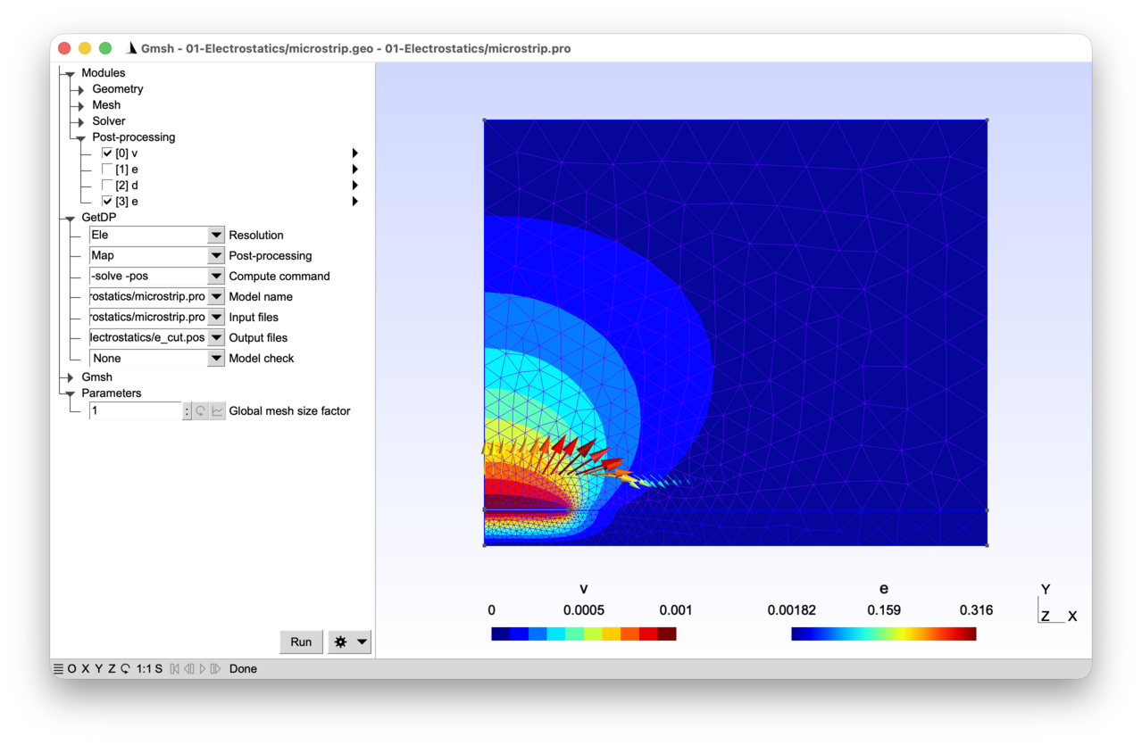
2.1 Tutorial 1: Electrostatic field around a microstrip line 
A 2D electrostatic model of a microstrip line is considered, with only one half of the geometry modelled by symmetry. A 1mV voltage is imposed on the microstrip line, which sits on top of a dielectric substrate grounded on its lower side.
2.1.1 Features 
- Electrostatic model in terms of the electric scalar potential
- Physical and abstract regions
- Scalar function space with Lagrange elements and Dirichlet constraint
See the comments in microstrip.pro and microstrip.geo for details.
2.1.2 Running the tutorial 
Each tutorial consists of (at least) two input files: a “.geo” file describing the geometry and the meshing constraints (the Gmsh part of the setup), and a “.pro” file describing the differential equations to solve together with the associated function spaces, boundary conditions and solver parameters (the GetDP part of the setup).
To run the tutorial on the command line:
> gmsh microstrip.geo -2
> getdp microstrip.pro -solve Ele -pos Map
To run the tutorial interactively with Gmsh: open microstrip.pro with “File->Open”, then press “Run”.
2.1.3 Contents 
File microstrip.geo 
// Gmsh script describing the geometry of the microstrip line and the associated
// meshing constraints.
//
// The microstrip line is a three-dimensional structure, but here we exploit the
// translation invariance along the line and model a 2D cross-section (a
// two-dimensional cut in a plane of constant "z"). All results are thus
// understood as values "per unit length along z".
//
// In this first tutorial we use the built-in Gmsh CAD kernel. Later tutorials
// (starting with tutorial 2) will use the more powerful OpenCASCADE kernel to
// build geometries from boolean operations on solid primitives.

// Dimensions (there are no units in Gmsh -- the following values should be
// interpreted as dimensions in meters due to the definition of the physical
// parameters in MKS units in "microstrip.pro"):
h = 1.e-3; // thickness of dielectric substrate
w = 4.72e-3; // width of microstrip line
t = 0.035e-3; // thickness of microstrip line
xBox = w/2. * 6.; // width of air box
yBox = h * 12.; // height of air box

// Global mesh size factor (that can be modified interactively in the Gmsh
// graphical interface):
s = DefineNumber[1., Name "Parameters/Global mesh size factor"];

// Target mesh sizes:
p0 = h / 10 * s;
pLine0 = w / 20 * s;
pLine1 = w / 100 * s;
pxBox = xBox / 10 * s;
pyBox = yBox / 8 * s;

// We create this first geometry in a bottom-up manner with the built-in Gmsh
// CAD kernel, successively defining model points, lines, loops and surfaces:
Point(1) = {0, 0, 0, p0};
Point(2) = {xBox, 0, 0, pxBox};
Point(3) = {xBox, h, 0, pxBox};
Point(4) = {0, h, 0, pLine0};
Point(5) = {w/2, h, 0, pLine1};
Point(6) = {0, h+t, 0, pLine0};
Point(7) = {w/2, h+t, 0, pLine1};
Point(8) = {0, yBox, 0, pyBox};
Point(9) = {xBox, yBox, 0, pyBox};
Line(1) = {1, 2};
Line(2) = {2, 3};
Line(3) = {3, 9};
Line(4) = {9, 8};
Line(5) = {8, 6};
Line(7) = {4, 1};
Line(8) = {5, 3};
Line(9) = {4, 5};
Line(10) = {6, 7};
Line(11) = {5, 7};
Curve Loop(12) = {1, 2, -8, -9, 7};
Plane Surface(13) = {12};
Curve Loop(14) = {10, -11, 8, 3, 4, 5};
Plane Surface(15) = {14};

// The last step is to define physical groups, assigning unique tags (and names)
// to groups of model entities. Physical groups serve two purposes: when they
// are defined they tell Gmsh which elements to save in the mesh file (by
// default only elements belonging to at least one physical group are saved),
// and they provide the tags that GetDP uses in "Region[]" to identify parts of
// the domain.
Physical Surface("Air", 1) = {15};
Physical Surface("Dielectric", 2) = {13};
Physical Curve("Ground", 10) = {1};
Physical Curve("Microstrip boundary", 11) = {9, 10, 11};
Physical Curve("Inf", 12) = {2, 3, 4};
File microstrip.pro 
// We consider the calculation of the electric field given a static distribution
// of electric potential. This corresponds to an electrostatic physical model,
// obtained by combining the time-invariant Faraday equation ("curl e = 0", with
// "e" the electric field) with Gauss' law ("div d = rho", with "d" the
// displacement field and "rho" the charge density) and the dielectric
// constitutive law ("d = epsilon e", with "epsilon" the dielectric
// permittivity).
//
// Since "curl e = 0", "e" can be derived from a scalar electric potential "v",
// such that "e = -grad v". Plugging this potential in Gauss' law and using the
// constitutive law leads to a scalar (generalized) Poisson equation in terms of
// the electric potential: "-div(epsilon grad v) = rho".
//
// We consider here the special case where "rho = 0" to model a conducting
// microstrip line on top of a dielectric substrate. A Dirichlet boundary
// condition sets the potential to 1 mV on the boundary of the microstrip line
// and to 0 V on the ground. A homogeneous Neumann boundary condition (zero
// normal component of the displacement field, i.e. "n . d = 0") is imposed on
// the left boundary of the domain to account for the symmetry of the problem. A
// homogeneous Neumann condition is also called a "natural" boundary condition:
// it appears in the weak formulation as a vanishing boundary integral, and
// therefore requires no explicit treatment in the model -- we simply do
// nothing. The domain is truncated on the top and right with a homogeneous
// Dirichlet boundary condition ("v = 0"), assumed to be imposed sufficiently
// far away from the microstrip.

Group {
  // Create region groups associated with the physical groups defined in the
  // "microstrip.msh" mesh file:
  Air = Region[ 1 ];
  Dielectric = Region[ 2 ];
  Ground = Region[ 10 ];
  Microstrip = Region[ 11 ];
  Inf = Region[ 12 ];

  // Define abstract regions to be used below in the definition of the scalar
  // electric potential formulation:
  //  - "Vol_Ele": overall volume domain where "-div(epsilon grad v) = 0" is
  //    solved; it contains only "volume" elements of the mesh (triangles here)
  //  - "Sur_Neu_Ele": surface where non homogeneous Neumann boundary conditions
  //    (on "n . d = -n . (epsilon grad v)") are imposed; it contain only
  //    "surface" elements of the mesh (lines here).
  //
  // The purpose of abstract regions is to allow a generic definition of the
  // FunctionSpace, Formulation and PostProcessing objects with no reference to
  // model-specific physical groups. We will show in tutorial 9 how abstract
  // formulations can then be isolated in geometry-independent template files,
  // thanks to an appropriate declaration mechanism (using "DefineConstant[]",
  // "DefineGroup[]" and "DefineFunction[]").
  //
  // Since there are no non-homogeneous Neumann conditions in this particular
  // example, "Sur_Neu_Ele" is defined as empty.
  //
  // Note that volume elements are those that correspond to the higher dimension
  // of the model at hand (2D elements here), surface elements correspond to the
  // higher dimension of the model minus one (1D elements here).
  Vol_Ele = Region[ {Air, Dielectric} ];
  Sur_Neu_Ele = Region[ {} ];
}

Function {
  // Material laws (here the dielectric permittivity) are defined as piecewise
  // functions (note the square brackets), in terms of the above defined groups:
  eps0 = 8.854187818e-12;
  epsilon[ Air ] = 1. * eps0;
  epsilon[ Dielectric ] = 9.8 * eps0;
}

Constraint {
  // The Dirichlet boundary condition is also defined piecewise, through the
  // following "v_Ele" constraint, invoked in the FunctionSpace below. The
  // constraint type "Assign" means that the coefficients in the finite element
  // expansion will be assigned the prescribed values:
  { Name v_Ele; Type Assign;
    Case {
      { Region Ground; Value 0.; }
      { Region Microstrip; Value 1.e-3; }
      { Region Inf; Value 0; }
    }
  }
}

Group{
  // The domain of definition of a FunctionSpace lists all regions on which a
  // field is defined. Domains of definitions may contain both volume and
  // surface regions, so we use a "Dom_" prefix to avoid confusion:
  Dom_H1_v_Ele =  Region[ {Vol_Ele, Sur_Neu_Ele} ];
}

FunctionSpace {
  // The function space in which we pick the electric scalar potential "v"
  // solution is defined by
  //  - a domain of definition (the "Support": "Dom_H1_v_Ele")
  //  - a type ("Form0", meaning "scalar field")
  //  - a set of basis functions ("BF_Node" for scalar nodal basis functions,
  //    i.e. isoparametric Lagrange elements)
  //  - a set of entities to which the basis functions are associated ("Entity":
  //    here all the nodes of the domain of definition "NodesOf[All]")
  //  - a constraint (here the Dirichlet boundary conditions)
  //
  // The finite element expansion of the unknown field "v" reads
  //
  //   v(x, y) = Sum_k vn_k sn_k(x, y)
  //
  // where the "vn_k" coefficients are the nodal values and "sn_k(x, y)" are the
  // nodal basis functions. Not all coefficients vn_k are unknowns of the finite
  // element problem, due to the Dirichlet constraint, which assigns particular
  // values to the nodes of the "Ground" and "Microstrip" regions.
  //
  // The default mesh "microstrip.msh" is made of first order (3-node)
  // triangles: the nodal basis functions sn_k(x, y) are then piece-wise linear
  // on each triangle. If second order (6-node) triangles are used instead
  // ("gmsh microstrip.geo -order 2 -2"), the basis functions will be piece-wise
  // quadratic on each triangle. In all cases, with Lagrange elements, we have
  // "sn_k(x_l, y_l) = \delta_kl" (the Kronecker delta, which is 1 if "k = l"
  // and 0 otherwise) if "(x_l, y_l)" denotes the coordinates of node "l".
  { Name H1_v_Ele; Type Form0;
    BasisFunction {
      { Name sn; NameOfCoef vn; Function BF_Node;
        Support Dom_H1_v_Ele; Entity NodesOf[ All ]; }
      // Using "NodesOf[All]" instead of "NodesOf[Dom_H1_v_Ele]" is an
      // optimization, which avoids explicitly building the list of all the
      // nodes. It is always safe here: GetDP restricts the actual basis
      // functions to those that have support in "Dom_H1_v_Ele". In cases where
      // different basis functions must be associated with disjoint subsets of
      // nodes (see e.g. tutorial 6), the explicit form "NodesOf[ <subset> ]"
      // becomes necessary.
    }
    Constraint {
      { NameOfCoef vn; EntityType NodesOf; NameOfConstraint v_Ele; }
    }
  }
}

Jacobian {
  // Jacobians specify the mapping between elements in the mesh and the
  // reference elements over which integration is performed.
  //
  // "Vol" stands for the 1-to-1 mapping between identical spatial dimensions,
  // i.e. in this case a reference triangle (2D) onto triangles in the "z = 0"
  // plane (2D):
  { Name Vol;
    Case {
      { Region All; Jacobian Vol; }
    }
  }
  // "Sur" is used to map the reference line segment (1D) onto lines in the
  // plane (2D). It is not strictly needed in this particular example (because
  // "Sur_Neu_Ele" is empty), but is defined here for completeness, so that
  // any surface term that might be added later to the Formulation (for
  // example the optional non-homogeneous Neumann term shown below) can
  // readily refer to it:
  { Name Sur;
    Case {
      { Region All; Jacobian Sur; }
    }
  }
}

Integration {
  // A Gauss numerical quadrature is used for the integrations:
  { Name Int;
    Case {
      { Type Gauss;
        Case {
          // One quadrature point is sufficient to integrate exactly the
          // stiffness matrix with first order elements (constant value per
          // element):
          { GeoElement Triangle; NumberOfPoints 1; }
          // But we need 3 quadrature points for second order elements:
          { GeoElement Triangle2; NumberOfPoints 3; }
        }
      }
    }
  }
}

Formulation {
  // The Formulation encodes the weak formulation of the original partial
  // differential equation, i.e. of "-div(epsilon grad v) = 0". This weak
  // formulation involves finding "v" such that
  //
  //   (-div(epsilon grad v) , v')_Vol_Ele = 0
  //
  // holds for all test functions "v'", where "(. , .)_D" denotes the inner
  // product over a domain "D". Integrating by parts (i.e. using Green's first
  // identity: "(div(f), u)_D = -(f, grad u)_D + (n . f, u)_Bnd_D"), the weak
  // formulation becomes: find "v" such that
  //
  //   (epsilon grad v, grad v')_Vol_Ele
  //     - (n . (epsilon grad v), v')_Bnd_Vol_Ele = 0
  //
  // holds for all "v'", where "Bnd_Vol_Ele" is the boundary of "Vol_Ele". In
  // our microstrip example this surface term vanishes, since
  //  - on the "Ground", "Microstrip" and "Inf" parts of the boundary we impose a
  //    Dirichlet boundary condition on "v" (through the "Assign" constraint)
  //    and the test functions "v'" vanish (there are actually none, as the
  //    corresponding unknowns have been fixed);
  //  - on the remaining part of the boundary (on the left side, at y = 0) by
  //    symmetry "n . d = - n. (epsilon grad v) = 0", i.e. we have a homogeneous
  //    Neumann ("natural") boundary condition.
  //
  // We are thus eventually looking for functions "v" in the function space
  // "H1_v_Ele" such that
  //
  //   (epsilon grad v, grad v')_Vol_Ele = 0
  //
  // holds for all "v'". Finally, our choice here is to use a Galerkin method,
  // where the test functions "v'" are the same basis functions ("sn_k") as the
  // ones used to interpolate the unknown potential "v".
  //
  // The "Integral" statement in the Formulation is a symbolic representation of
  // this weak formulation. It has 4 semicolon separated arguments:
  //  - the density "[. , .]" to be integrated (note the square brackets instead
  //    of the parentheses), with the test functions (always) after the comma;
  //  - the domain of integration;
  //  - the Jacobian of the transformation between the reference element and the
  //    element in the mesh;
  //  - the integration method.
  //
  // In the density, braces around a quantity (such as "{v}") indicate that this
  // quantity belongs to a FunctionSpace. Differential operators can be applied
  // within braces (such as "{Grad v}"); in particular the symbol "d" represents
  // the exterior derivative, and it is a synonym of "Grad" when applied to a
  // scalar function, declared with type "Form0" in the FunctionSpace.
  //
  // As the Galerkin method uses as test functions the same basis functions
  // "sn_k" as for the unknown field "v", the second term in the density should
  // be something like [ ... , basis_functions_of {d v} ]. However, since the
  // second term is always devoted to test functions, the operator
  // "basis_functions_of" would always be there.  It can therefore be made
  // implicit and, in the GetDP syntax, it is omitted. So, one simply writes "[
  // ... , {d v} ]".
  //
  // On the other hand, the first term can contain a much wider variety of
  // expressions. In our case it should be expressed in terms of the finite
  // element expansion of "v" at the present system solution, i.e. when the
  // coefficients "vn_k" in the expansion "v = Sum_k vn_k sn_k" are
  // unknown. This is indicated by prefixing the braces with "Dof" ("degree of
  // freedom"), which leads to the following density:
  //
  //   [ epsilon[] * Dof{d v} , {d v} ],
  //
  // a bilinear term that will contribute to the stiffness matrix of the
  // electrostatic problem at hand.
  //
  // Another option, which does not work here (because it would make the
  // problem trivial: there would be no unknowns left), is to evaluate the
  // first argument with the last available computed solution, i.e. simply
  // perform the interpolation with known coefficients "vn_k". The "Dof"
  // prefix is then omitted and we would have:
  //
  //   [ epsilon[] * {d v} , {d v} ],
  //
  // a linear term that would contribute to the right-hand side of the linear
  // system. This mechanism is not useful for a linear, one-shot problem like
  // the present one, but it is essential whenever a term depends on a
  // previously computed field: see tutorial 3 (where the reluctivity "nu" is
  // evaluated at the current iterate "{d a}" inside a Newton-Raphson loop)
  // and tutorial 7 (where the electrical conductivity is evaluated at the
  // temperature field "{T}" computed by a separate formulation).

  { Name Electrostatics_v; Type FemEquation;
    Quantity {
      { Name v; Type Local; NameOfSpace H1_v_Ele; }
    }
    Equation {
      Integral { [ epsilon[] * Dof{d v} , {d v} ];
        In Vol_Ele; Jacobian Vol; Integration Int; }

      // Additional "Integral" terms can be added here. For example, the
      // following term may account for non-homogeneous Neumann boundary
      // conditions, provided that the function "nd[]" is defined:
      //
      // Integral { [ nd[] , {v} ];
      //   In Sur_Neu_Ele; Jacobian Sur; Integration Int; }

      // All the terms in the "Equation" are added, and an implicit "= 0" is
      // considered at the end.
    }
  }
}

// In "Resolution" we specify what to do with a weak formulation: here we simply
// generate a linear system, solve it and save the solution to disk (in a ".res"
// file).
Resolution {
  { Name Ele;
    System {
      { Name Sys_Ele; NameOfFormulation Electrostatics_v; }
    }
    Operation {
      Generate[Sys_Ele]; Solve[Sys_Ele]; SaveSolution[Sys_Ele];
    }
  }
}

// Post-processing is done in two parts.
//
// The first part defines, in terms of the Formulation, which itself refers to
// the FunctionSpace, a number of quantities that can be evaluated at the
// post-processing stage. The three quantities defined here are:
//  - the scalar electric potential;
//  - the electric field;
//  - the electric displacement.
PostProcessing {
  { Name Ele; NameOfFormulation Electrostatics_v;
    Quantity {
      { Name v; Value {
          Term { [ {v} ]; In Vol_Ele; Jacobian Vol; }
        }
      }
      { Name e; Value {
          Term { [ -{d v} ]; In Vol_Ele; Jacobian Vol; }
        }
      }
      { Name d; Value {
          Term { [ -epsilon[] * {d v} ]; In Vol_Ele; Jacobian Vol; }
        }
      }
    }
  }
}

// The second part consists in defining post-processing operations, which can be
// invoked separately. (The first PostOperation is invoked by default when Gmsh
// is run interactively. The generated post-processing files are automatically
// displayed by Gmsh if the "Merge result automatically" option is enabled in
// the Gmsh "gear" menu.)

tol = 1.e-7; // small offset to ensure the cut is inside the simulation domain
yCut = 2.e-3; // vertical position of the cut

PostOperation {
  { Name Map; NameOfPostProcessing Ele;
     Operation {
       Print [ v, OnElementsOf Vol_Ele, File "v.pos" ];
       Print [ e, OnElementsOf Vol_Ele, File "e.pos" ];
       Print [ d, OnElementsOf Vol_Ele, File "d.pos" ];
       Print [ e, OnLine {{tol, yCut, 0}{14.e-3, yCut, 0}}{60}, File "e_cut.pos" ];
     }
  }
  { Name Cut; NameOfPostProcessing Ele;
    // Same cut as above, with more points and exported in raw text format.
    // "Format Table" requests an ASCII file (one row of numbers per evaluation
    // point) instead of the default Gmsh ".pos" format, which carries mesh
    // information and is automatically rendered by Gmsh. A ".txt" file is
    // primarily intended for post-processing by external tools (spreadsheets,
    // plotting scripts, etc.).
    //
    // Note that PostOperations other than the default one are invoked from the
    // Gmsh GUI through the "Modules > GetDP > Post-processing" menu (or from
    // the command line, e.g. with "getdp microstrip.pro -solve Ele -pos Cut"):
    Operation {
      Print [ e, OnLine {{tol, tol, 0}{14.e-3, tol, 0}} {500}, Format Table,
        File "e_cut.txt" ];
    }
  }
}
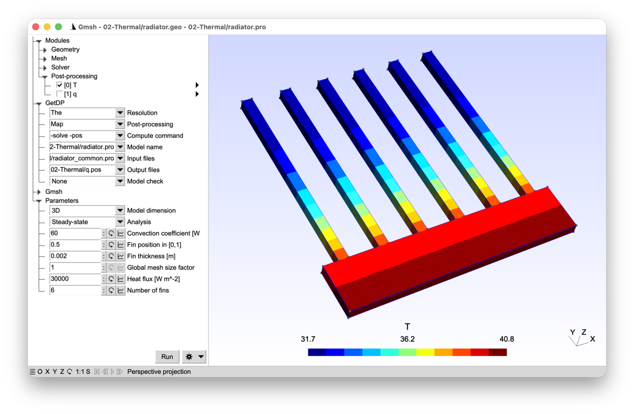
2.2 Tutorial 2: Thermal conduction in a radiator with fins 
A 2D and 3D thermal model of an aluminum radiator is considered. A heat flux is applied to the bottom of the base plate of the radiator, while convection is modelled using Newton’s law of cooling on the radiator fins. Periodic boundary conditions allow the simulation of non-symmetric elementary radiator cells. Both steady-state and transient simulations can be performed.
2.2.1 Features 
- Thermal model with conduction and convection
- Two- and three-dimensional models
- Steady-state and transient simulations
- Neumann, Robin and periodic boundary conditions
See the comments in radiator.pro and radiator.geo for details.
2.2.2 Running the tutorial 
On the command line (2D analysis):
> gmsh radiator.geo -2
> getdp radiator.pro -solve The -pos Map
On the command line (3D analysis):
> gmsh radiator.geo -3 -setnumber dim 3
> getdp radiator.pro -solve The -pos Map -setnumber dim 3
Interactively with Gmsh: open radiator.pro with “File->Open”, then press “Run”.
2.2.3 Contents 
File radiator_common.pro 
bw = 8e-3; // base plate width (for one fin)
DefineConstant[
  N = {1, Min 1, Max 100, Step 1, Name "Parameters/Number of fins"}
];
File radiator.geo 
// Gmsh script describing the geometry of the radiator and the associated
// meshing constraints.

// Instead of the built-in Gmsh geometry kernel we use the OpenCASCADE kernel,
// in order to benefit from boolean operations:
SetFactory("OpenCASCADE");

// Definition of a global mesh size factor that can be modified interactively in
// the Gmsh graphical interface (in the same way as with DefineNumber[] - see
// tutorial 1), but that can also be overridden beforehand, e.g. on the command
// line with "-setnumber s value":
DefineConstant[
  s = {1., Name "Parameters/Global mesh size factor"}
];

fh = 40e-3; // fin height
fw = 2e-3; // fin width
bh = 10e-3; // base plate height
lc = fw / 3 * s; // mesh size

// We include a file that defines the number of fins and the width of one cell:
// the same file will be included in radiator.pro to guarantee consistency
// between Gmsh and GetDP when defining the periodic boundary condition
Include "radiator_common.pro";

DefineConstant[
  position = {0.5, Min 0.1, Max 0.9, Step 0.1,
    Name "Parameters/Fin position in [0,1]"}
  dim = {2, Choices{2="2D", 3="3D"},
    Name "Parameters/0Model dimension"}
  zh = {fh / 20, Min 1e-3, Max 2 * fh, Step 1e-3, Visible dim == 3,
    Name "Parameters/Fin thickness [m]"}
];

For i In {0 : N - 1}
  x0 = i * bw;
  Rectangle(2 * i + 1) = {x0 + position * (bw - fw), bh, 0, fw, fh}; // fin
  Rectangle(2 * i + 2) = {x0, 0, 0, bw, bh}; // base plate
EndFor

surf() = BooleanUnion{ Surface{1}; Delete; }{ Surface{2 : 2 * N}; Delete; };

MeshSize{:} = lc;

// Note that a number prefix in a parameter name is invisible in the graphical
// user interface ("0Model dimension" will appear as "Model dimension"). It
// enables sorting the menu entries, i.e. in this case making sure that "Model
// dimension" is the first entry in the "Parameters" menu.

e = 1e-6; // small tolerance for bounding box searches below

If(dim == 2)
  interior = surf(0);
  bottom() = Curve In BoundingBox{-e, -e, -e, N * bw + e, e, e};
  left() = Curve In BoundingBox{-e, -e, -e, e, bh + e, e};
  right() = Curve In BoundingBox{N * bw - e, -e, -e, N * bw + e, bh + e, e};
  top() = Boundary{ Surface{interior}; };
  top() -= {bottom(), left(), right()};

  // Set a periodic mesh constraint on the right curve: this forces Gmsh to
  // generate identical meshes on the "right" and "left" boundaries (the nodes
  // and elements of one are obtained from those of the other by the prescribed
  // translation). This matching of the two meshes is what enables the "Link"
  // constraint defined in "radiator.pro" to connect the degrees of freedom of
  // the two boundaries node-by-node:
  Periodic Curve { right() } = { left() } Translate {N * bw, 0, 0};
Else
  ex() = Extrude {0, 0, zh}{ Surface{surf()}; };
  interior = ex(1);
  bottom() = Surface In BoundingBox{-e, -e, -e, N * bw + e, e, zh + e};
  left() = Surface In BoundingBox{-e, -e, -e, e, bh + e, zh + e};
  right() = Surface In BoundingBox{N * bw - e, -e, -e, N * bw + e, bh + e, zh + e};
  top() = Boundary{ Volume{interior}; };
  top() -= {bottom(), left(), right()}; // try adding e.g. surf() and ex(0)

  // Set a periodic mesh constraint on the right surface (same purpose as in
  // the 2D case above):
  Periodic Surface { right() } = { left() } Translate {N * bw, 0, 0};
EndIf

// Define physical groups (GeoEntity{dim} can be used as a synonym for Curve,
// Surface and Volume respectively for dim == 1, 2 and 3):
Physical GeoEntity{dim} ("Radiator", 1) = interior;
Physical GeoEntity{dim - 1} ("Bottom base plate", 10) = bottom();
Physical GeoEntity{dim - 1} ("Left base plate", 11) = left();
Physical GeoEntity{dim - 1} ("Right base plate", 12) = right();
Physical GeoEntity{dim - 1} ("Top fins", 13) = top();
File radiator.pro 
// This model computes the temperature profile in a radiator with fins.
// Starting at an initial temperature "T = T0", a heat flux "qn = qn0" is
// imposed through the bottom surface of the radiator base plate. Convection on
// the fins evacuates the heat based on Newton's law of cooling "qn = h (T -
// T0)", with "h" the convection coefficient.
//
// The governing partial differential equation links the temperature "T" and the
// heat flux density vector "q" through
//
//   rho * cp * \partial_t T + div(q) = 0,
//
// where "rho" is the mass density and "cp" the specific heat. Introducing
// Fourier's law "q = -k grad T", with "k" the thermal conductivity, we get the
// heat diffusion equation in terms of the temperature:
//
//   rho * cp * \partial_t T - div(k grad T) = 0.
//
// We will see below that the heat flux will be imposed naturally through a
// non-homogeneous Neumann boundary condition, while the convection condition
// will be imposed through a Robin boundary condition.

Group {
  // Physical regions:
  Radiator = Region[ 1 ];
  Bottom = Region[ 10 ];
  Left = Region[ 11 ];
  Right = Region[ 12 ];
  Top = Region[ 13 ];

  // The abstract regions in this model have the following interpretation:
  //  - "Vol_The": overall domain
  //  - "Sur_Neu_The": part of the boundary with non-homogeneous Neumann
  //    condition
  //  - "Sur_Rob_The": part of the boundary with Robin condition
  Vol_The = Region[ {Radiator} ];
  Sur_Neu_The = Region[ {Bottom} ];
  Sur_Rob_The = Region[ {Top} ];
}

Function {
  // "DefineConstant[]" declares parameters that can be modified interactively
  // in the Gmsh GUI, or overridden on the command line with "-setnumber name
  // value":
  DefineConstant[
    AnalysisType = {0, Choices{0="Steady-state", 1="Transient"},
      Name "Parameters/Analysis"}
    qn0 = {3e4, Min 1, Max 1e6, Step 1e3,
      Name "Parameters/Heat flux [W m^-2]"}
    h = {60, Min 0, Max 120, Step 1,
      Name "Parameters/Convection coefficient [W m^-2 K^-1]"}
    tmax = {360, Min 1, Max 3600, Step 10,
      Name "Parameters/Simulation time [s]", Visible AnalysisType}
    dt = {5, Min 0.1, Max 100, Step 0.1,
      Name "Parameters/Time step [s]", Visible AnalysisType}
  ];

  rho_cp[] = 2700 * 900;
  k[] = 170;
  qn0[] = -qn0; // negative sign to have flux coming into "Vol_The"
  h[] = h;
  T0[] = 20;
}

// The weak formulation reads: find "T" such that
//
//   (rho * cp * \partial_t T, T')_Vol_The - (div(k grad T), T')_Vol_The = 0
//
// holds for all test functions "T'". After integration by parts it reads: find
// "T" such that
//
//   (rho * cp * \partial_t T, T')_Vol_The + (k grad T, grad T')_Vol_The
//     - (k grad T . n, T')_Bnd_Vol_The = 0
//
// holds for all test functions "T'". The boundary term is split to handle the
// imposed flux ("-k grad T . n = qn0") as a non-homogeneous Neumann boundary
// condition on "Sur_Neu_The", and the convection condition ("-k grad T . n = h
// (T - T0)") as a Robin condition on "Sur_Rob_The". The final weak formulation
// then reads: find "T" such that
//
//   (rho * cp * \partial_t T, T')_Vol_The + (k grad T, grad T')_Vol_The
//     + (qn0, T')_Sur_Neu_The + (h (T - T0), T')_Sur_Rob_The = 0
//
// holds for all test functions "T'".
//
// In the steady-state, the first term vanishes. Note that this problem is still
// well-posed, even without Dirichlet boundary conditions, thanks to the Robin
// condition (with "h > 0"). Indeed, the bilinear form is coercive: "a(T, T) =
// \int_Vol_The k |grad T|^2 + \int_Sur_Rob_The h T^2 >= C ||T||^2_H1".

Jacobian {
  { Name Vol;
    Case {
      { Region All; Jacobian Vol; }
    }
  }
  { Name Sur;
    Case {
      { Region All; Jacobian Sur; }
    }
  }
}

Integration {
  { Name Int;
    Case {
      { Type Gauss;
        Case {
          // We need to integrate on lines and triangles for the 2D model, and
          // on triangles and tetrahedra for the 3D model. We need sufficiently
          // many quadrature points to integrate quadratic functions (inner
          // product "(T , T')" of piecewise linear functions):
          { GeoElement Line; NumberOfPoints 2; }
          { GeoElement Triangle; NumberOfPoints 3; }
          { GeoElement Tetrahedron; NumberOfPoints 4; }
        }
      }
    }
  }
}

// Include definitions needed for the Link constraint below:
Include "radiator_common.pro";

Constraint {
  { Name T_The;
    Case {
      // Initial condition for transient solution (different constraint types
      // can be specified for each region within the "Case" -- compare with the
      // global "Type Assign" used in tutorial 1):
      If(AnalysisType == 1)
        { Region Vol_The; Type Init; Value T0[]; }
      EndIf
      // For a symmetric geometry (with position = 0.5 in "radiator.geo") a
      // homogeneous Neumann boundary condition on the Left and Right boundaries
      // is sufficient to ensure periodicity. Otherwise an explicit periodicity
      // condition is required. This can be achieved in GetDP with a "Link"
      // constraint, which links degrees of freedom from two regions ("Region"
      // and "RegionRef", geometrically mapped onto each other with "Function"),
      // with a coefficient. This requires the mesh to match on both regions.
      { Region Right; Type Link; RegionRef Left; Coefficient 1;
        // The function maps Region onto RegionRef, using the built-in "X[]",
        // "Y[]", "Z[]" coordinate functions to define the translation vector:
        Function Vector[X[] - N * bw, Y[], Z[]]; }
    }
  }
}

Group{
  Dom_H1_T_The =  Region[ {Vol_The, Sur_Neu_The, Sur_Rob_The} ];
}

FunctionSpace {
  { Name H1_T_The; Type Form0;
    BasisFunction {
      { Name sn; NameOfCoef Tn; Function BF_Node; Support Dom_H1_T_The;
        Entity NodesOf[All]; }
    }
    Constraint {
      { NameOfCoef Tn; EntityType NodesOf; NameOfConstraint T_The; }
    }
  }
}

Formulation {
  { Name Thermal_T; Type FemEquation;
    Quantity {
      { Name T; Type Local; NameOfSpace H1_T_The; }
    }
    Equation {
      // A "DtDof" term enables GetDP to handle time discretization
      // automatically (depending on the operation) in a "Resolution":
      Integral { DtDof [ rho_cp[] * Dof{T} , {T} ];
        In Vol_The; Jacobian Vol; Integration Int; }

      Integral { [ k[] * Dof{d T} , {d T} ];
        In Vol_The; Jacobian Vol; Integration Int; }

      Integral { [ qn0[] , {T} ];
        In Sur_Neu_The; Jacobian Sur; Integration Int; }

      // In GetDP equation terms with "Dof" must be linear with respect to the
      // value of the degree of freedom, so a "Dof" term with an affine part
      // such as "[ h[] * (Dof{T} - T0[]), {T} ]" is invalid and must be split
      // into two separate terms:
      Integral { [ h[] * Dof{T} , {T} ];
        In Sur_Rob_The; Jacobian Sur; Integration Int; }
      Integral { [ -h[] * T0[] , {T} ];
        In Sur_Rob_The; Jacobian Sur; Integration Int; }
    }
  }
}

Resolution {
  { Name The;
    System {
      { Name Sys_The; NameOfFormulation Thermal_T; }
    }
    Operation {
      If(AnalysisType == 1) // Transient
        // Initialize the solution:
        InitSolution[Sys_The];
        // Perform a time loop with an implicit Euler scheme, from time == 0 to
        // time == "tmax", with fixed time step "dt":
        TimeLoopTheta[0, tmax, dt, 1] {
          Generate[Sys_The]; Solve[Sys_The]; SaveSolution[Sys_The];
        }
        // More advanced time discretizations are available as built-in
        // resolution operations (see e.g. "TimeLoopAdaptive"). They could also be
        // implemented manually by replacing the "DtDof" term in the formulation
        // with the chosen approximation, e.g.
        //
        //   Integral { [ rho_cp[] * Dof{T} / dt, {T} ];
        //     In Vol_The; Integration Int; Jacobian Vol;  }
        //   Integral { [ - rho_cp[] * {T}[1] / dt, {T} ];
        //     In Vol_The; Integration Int; Jacobian Vol;  }
        //
        // for implicit Euler ("{T}[1]" denotes the value of "{T}" at the
        // previous step). A custom time integration loop can then be
        // constructed in the resolution with the "While[]" operation.
      Else // Steady-state
        // The "DtDof" term is automatically disregarded by GetDP if there is no
        // time loop, so we can generate and solve the steady-state system
        // directly:
        Generate[Sys_The]; Solve[Sys_The]; SaveSolution[Sys_The];
      EndIf
    }
  }
}

PostProcessing {
  { Name The; NameOfFormulation Thermal_T;
    Quantity {
      { Name T; Value{ Local{ [ {T} ]; In Vol_The; Jacobian Vol;} } }
      { Name q; Value{ Local{ [ -k[] * {d T} ]; In Vol_The; Jacobian Vol; } } }
    }
  }
}

PostOperation {
  { Name Map; NameOfPostProcessing The;
    Operation {
      Print[ T, OnElementsOf Vol_The, File "T.pos"];
      Print[ q, OnElementsOf Vol_The, File "q.pos"];
    }
  }
}
2.3 Tutorial 3: Magnetostatic model of an electromagnet 
A 2D magnetostatic model of an electromagnet is considered. A current density is imposed in the coil, and the ferromagnetic core can be modelled either using a linear or a nonlinear constitutive law. Infinite elements are used to accurately model the unbounded domain.

2.3.1 Features 
- Magnetostatic model in terms of the magnetic vector potential
- Infinite ring geometrical transformation
- Function space for the 2D vector potential (“perpendicular edges”)
- Newton-Raphson and Picard linearization schemes
See the comments in electromagnet.pro and electromagnet.geo for details.
2.3.2 Running the tutorial 
On the command line:
> gmsh electromagnet.geo -2
> getdp electromagnet.pro -solve Mag -pos Map
Interactively with Gmsh: open electromagnet.pro with “File->Open”, then press “Run”.
2.3.3 Contents 
File electromagnet_common.pro 
// Parameters shared by Gmsh and GetDP.

mm = 1e-3;

dxCore = 50 * mm;
dyCore = 100 * mm;
xCoil = 75 * mm;
dxCoil = 25 * mm;
dyCoil = 100 * mm;
rInt = 200 * mm;
rExt = 250 * mm;

DefineConstant[
  SymmetryType = {0, Choices{0="None", 1="X-axis", 2="Y-axis", 3="All"},
    Name "Parameters/0Symmetry"}
];
File electromagnet.geo 
// Gmsh script describing the geometry of an electromagnet with an iron core and
// two coil sides, surrounded by air. The 3D setup is invariant along the
// out-of-plane direction "z" (the axis of the coils), so we model a 2D
// cross-section in the "(x, y)" plane. The two additional symmetries of this
// cross-section -- with respect to the X-axis (separating the two coil sides)
// and to the Y-axis (passing through the core) -- make it possible to model
// only a half (or even a quarter) of the cut. The "SymmetryType" parameter
// defined in "electromagnet_common.pro" selects which part is meshed.
//
// Note: tutorial 1 used the built-in Gmsh CAD kernel. Here we switch to
// OpenCASCADE, which offers boolean operations on solid primitives.

// We include a file with the dimensions as well as the symmetry type; the same
// file will be included in electromagnet.pro to guarantee consistency between
// Gmsh and GetDP:
Include "electromagnet_common.pro";

SetFactory("OpenCASCADE");
Rectangle(1) = {-dxCore, -dyCore, 0, 2 * dxCore, 2 * dyCore};
Rectangle(2) = {xCoil, -dyCoil / 2, 0, dxCoil, dyCoil};
Rectangle(3) = {-xCoil - dxCoil, -dyCoil / 2, 0, dxCoil, dyCoil};
Disk(4) = {0, 0, 0, rInt};
Disk(5) = {0, 0, 0, rExt};

If(SymmetryType == 0) // no symmetry
  // With the OpenCASCADE kernel the "Coherence" command is a shortcut for
  // "BooleanFragments" applied to all entities of the highest dimension. It
  // computes the intersections of all overlapping entities and replaces them
  // with a conformal (non-overlapping) set of entities. This is essential when
  // building a geometry from overlapping primitives with the OpenCASCADE
  // kernel: without it, entities would overlap and the resulting mesh would not
  // be conformal at region interfaces. After "Coherence" each original primitive
  // has been fragmented into the pieces that actually belong to each physical
  // region (core, coils, air, infinite shell), which is what the "Closest"
  // queries below rely on to retrieve them by position.
  Coherence;
Else
  // A bounding rectangle is built and intersected with the previously defined
  // primitives. The three non-trivial values of "SymmetryType" are handled
  // uniformly by the following formulas:
  //   - SymmetryType == 1: keep the upper half (y >= 0), X-axis is a symmetry
  //     plane, so "bot()" later carries the "n x h = 0" boundary condition;
  //   - SymmetryType == 2: keep the right half (x >= 0), Y-axis is a symmetry
  //     plane, so "left()" later carries the "b . n = 0" boundary condition;
  //   - SymmetryType == 3: keep the first quadrant (x >= 0 and y >= 0), both
  //     axes are symmetry planes, so both "bot()" and "left()" are defined
  //     below.
  d = 1.1 * rExt;
  x = (SymmetryType == 1) ? -d : 0; // symmetry w.r.t. X-axis ?
  dx = (SymmetryType == 1) ? 2 * d : d;
  y = (SymmetryType == 2) ? -d : 0; // symmetry w.r.t. Y-axis ?
  dy = (SymmetryType == 2) ? 2 * d : d;
  Rectangle(6) = {x, y, 0, dx, dy};
  BooleanIntersection{ Surface{6}; Delete; }{ Surface{1:5}; Delete; }
EndIf

// After boolean operations the original surface tags may have changed. The
// "Closest" command retrieves the entities closest to a given point, sorted by
// distance, which is a convenient way to identify the desired surfaces by their
// geometric location -- it is enough that the probe point lies inside the target
// region to retrieve it unambiguously:
core() = Closest{0, 0, 0}{ Surface{:}; };
air() = Closest{dxCore + mm, 0, 0}{ Surface{:}; };
airinf() = Closest{rInt + mm, 0, 0}{ Surface{:}; };
indr() = Closest{xCoil + mm, 0, 0}{ Surface{:}; };
indl() = Closest{-xCoil - mm, 0, 0}{ Surface{:}; };
Physical Surface("Core", 1) = core(0);
Physical Surface("Air", 2) = air(0);
Physical Surface("AirInf", 3) = airinf(0);
Physical Surface("CoilRight", 4) = indr(0);
If(SymmetryType == 0 || SymmetryType == 1)
  Physical Surface("CoilLeft", 5) = indl(0);
EndIf

bot() = {};
left() = {};
If(SymmetryType == 1 || SymmetryType == 3)
  bot() = Curve In BoundingBox{-d, -mm, -mm, d, mm, mm};
  Physical Curve("Bottom", 10) = bot();
EndIf
If(SymmetryType == 2 || SymmetryType == 3)
  left() = Curve In BoundingBox{-mm, -d, -mm, mm, d, mm};
  Physical Curve("Left", 11) = left();
EndIf

inf() = CombinedBoundary{ Surface{:}; };
inf() -= {bot(), left()};
Physical Curve("Inf", 12) = inf();

// Mesh size constraints:
DefineConstant[
  s = {1, Name "Parameters/}Global mesh size factor"}
];

MeshSize{:} = 12.5 * mm * s;
MeshSize{ PointsOf{ Surface{indr(0)}; } } = 5 * mm * s;
If(SymmetryType == 0 || SymmetryType == 1)
  MeshSize{ PointsOf{ Surface{indl(0)}; } } = 5 * mm * s;
EndIf
MeshSize{ PointsOf{ Surface{core(0)}; } } = 4 * mm * s;
File electromagnet.pro 
// This model computes the static magnetic field produced by a DC current in an
// electromagnet. This corresponds to a magnetostatic physical model, obtained
// by combining the time-invariant Maxwell-Ampere equation ("curl h = js", with
// "h" the magnetic field and "js" the source current density) with the magnetic
// Gauss law ("div b = 0", with "b" the magnetic flux density) and the magnetic
// constitutive law ("b = mu h", with "mu" the magnetic permeability).
//
// Since "div b = 0", "b" can be derived from a vector magnetic potential "a",
// such that "b = curl a". Plugging this vector potential in Maxwell-Ampere's
// law and using the constitutive law leads to a generalized vector Poisson
// equation in terms of the magnetic vector potential: "curl(nu curl a) = js",
// where "nu = 1/mu" is the magnetic reluctivity.
//
// In the general (3D) case the vector potential is not unique, since for all
// scalar functions "f", "b = curl a = curl (a + grad f)". We will introduce
// explicit gauge conditions in tutorial 8 and 10 to ensure uniqueness. In the
// 2D setting however, with a source current density along the z-axis, the
// magnetic vector potential "a" is a vector field with a single non-zero
// component along the z-axis, i.e.:
//
//   a = (0, 0, az(x, y))
//
// which automatically removes gradient fields from the admissible space (the
// kernel reduces to constants, which a Dirichlet boundary condition is
// sufficient to fix).
//
// Magnetostatic fields expand to infinity. The corresponding boundary condition
// can be imposed rigorously by means of a geometrical transformation that maps
// a ring (a "shell") of finite elements to the complementary of its interior.
// As this is a mere geometric transformation, it is enough in the model
// description to attribute the special Jacobian "VolSphShell" to the ring
// region "AirInf". This Jacobian takes as arguments the inner ("rInt") and
// outer ("rOut") radii of the transformed ring region: to ensure consistency
// they are defined in a separate file, which is included in both the .geo and
// .pro file.  For a derivation and discussion of this transformation technique,
// see e.g. F. Henrotte et al., "Finite element modelling with transformation
// techniques", IEEE Transactions on Magnetics, 35(3), 1434-1437, 1999.

Include "electromagnet_common.pro";

// With this information, GetDP is able to correctly transform all quantities
// involved in the model. The model exhibits two symmetries: with respect to the
// X-axis and with respect to the Y-axis. The "SymmetryType" constant defined in
// "electromagnet_common.pro" allows to solve the problem with or without taking
// advantage of them.

Group {
  // Physical regions:
  Core = Region[ 1 ];
  Air = Region[ 2 ];
  AirInf = Region[ 3 ];
  CoilRight = Region[ 4 ];
  // Left coil only if no symmetry, or if single symmetry with respect to X-axis:
  CoilLeft = Region[ {} ];
  If(SymmetryType == 0 || SymmetryType == 1)
    CoilLeft += Region[ 5 ];
  EndIf
  Coils = Region[ {CoilLeft, CoilRight} ];
  // Bottom boundary only if symmetry with respect to X-axis:
  Bottom = Region[ {} ];
  If(SymmetryType == 1 || SymmetryType == 3)
    Bottom += Region[ 10 ];
  EndIf
  // Left boundary only if symmetry with respect to Y-axis:
  Left = Region[ {} ];
  If(SymmetryType == 2 || SymmetryType == 3)
    Left += Region[ 11 ];
  EndIf
  Inf = Region[ 12 ];

  // The abstract regions in this model have the following interpretation:
  //  - "Vol_Mag": overall domain
  //  - "Vol_S_Mag": region with imposed current source js
  //  - "Vol_NL_Mag": region with nonlinear magnetic constitutive law
  //  - "Vol_L_Mag": region with linear magnetic constitutive law
  //  - "Vol_Inf_Mag": region with infinite shell geometric transformation
  //  - "Sur_Neu_Mag": part of the boundary with non-homogeneous Neumann
  //    conditions
  Vol_Mag = Region[ {Air, AirInf, Core, Coils} ];
  Vol_S_Mag = Region[ Coils ];
  Vol_Inf_Mag = Region[ AirInf ];
  Sur_Neu_Mag = Region[ {} ]; // empty

  DefineConstant[
    NonlinearCore = {0, Choices {0, 1},
      Help "Is the magnetic law in the core nonlinear?",
      Name "Parameters/Nonlinear core"}
  ];

  If(NonlinearCore)
    Vol_NL_Mag = Region[ Core ];
  Else
    Vol_NL_Mag = Region[ {} ];
  EndIf
  // "-" to subtract "Vol_NL_Mag" from "Vol_Mag". "Vol_L_Mag" is therefore the
  // linear part of the magnetic domain: in the linear case it coincides with
  // the full domain, and in the nonlinear case it is everything except the
  // (nonlinear) core:
  Vol_L_Mag = Region[ {Vol_Mag, -Vol_NL_Mag} ];
}

// The weak formulation is derived in a similar way as for the electrostatic or
// thermal problems from previous tutorials. The main differences are that the
// unknown field is vector-valued, and that we want to handle the nonlinear case
// when nu is not constant. The weak formulation reads: find "a" such that
//
//   (curl(nu curl a), a')_Vol_Mag = (js, a')_Vol_S_Mag
//
// holds for all test functions "a'". After integration by parts it reads: find
// "a" such that
//
//   (nu curl a, curl a')_Vol_Mag + (n x (nu curl a), a')_Bnd_Vol_Mag =
//      (js, a')_Vol_S_Mag
//
// holds for all test functions "a'". In the electromagnet model the second
// (boundary) term vanishes:
//
//  - On the "Left" and "Inf" parts of the boundary, the normal component of "b"
//    must vanish by symmetry and decay, respectively. Imposing "a = 0" there
//    (homogeneous Dirichlet) enforces "b . n = 0" (since the tangential "a" is
//    zero, the flux of "b" through any surface patch on the boundary is zero by
//    Stokes' theorem). The boundary term vanishes because the test functions
//    "a'" are zero there -- GetDP automatically removes the corresponding test
//    functions when an "Assign" constraint is prescribed. For the "Left" part
//    of the 2D planar model, the "a = 0" condition can also be understood
//    directly: by symmetry with respect to the Y-axis the magnetic vector
//    potential has opposite signs on either side (the current density that
//    sources it is antisymmetric); continuity then forces "az = 0" on the axis
//    itself.
//
//  - On the "Bottom" boundary, the tangential component of "h" is zero by
//    symmetry, i.e. "n x h = n x (nu curl a) = 0". This is a homogeneous
//    Neumann condition: it is satisfied naturally (the boundary integrand is
//    zero).
//
// Note that depending on the value of "SymmetryType", the "Left" and/or
// "Bottom" region might be empty.
//
// We are thus eventually looking for functions a such that
//
//   (nu curl a, curl a')_Vol_Mag = (js, a')_Vol_S_Mag
//
// holds for all test functions "a'".
//
// If the magnetic constitutive law is nonlinear, i.e. if "nu" is not a constant
// but a function of "b = curl a", we need to linearize the formulation before
// we can solve it in GetDP. Several linearization methods are possible:
//
// 1) Newton-Raphson method - at iteration "k" we approximate
//
//   h(b_k) \approx h(b_k-1) + (dh/db)_k-1 (b_k - b_k-1)
//
// i.e.
//
//   (nu(curl a_k) curl a_k, curl a')
//     \approx (nu(curl a_k-1) curl a_k-1, curl a')
//           + (dh/db(curl a_k-1) curl a_k, curl a')
//           - (dh/db(curl a_k-1) curl a_k-1, curl a')
//
// 2) Picard method - at iteration "k" we approximate
//
//   (nu(curl a_k) curl a_k, curl a')
//     \approx (nu(curl a_k-1) curl a_k, curl a')

Function {
  DefineConstant[
    NewtonRaphson = {1, Choices {0="Picard", 1="Newton-Raphson"},
      Visible NonlinearCore,
      Name "Parameters/Linearization method"}
    Current = {1, Min 0.01, Max 100, Step 0.1,
      Name "Parameters/Current [A]"}
  ];

  mu0 = 4.e-7 * Pi;
  nu0 = 1 / mu0;
  nu [ Air ] = nu0;
  nu [ AirInf ] = nu0;
  nu [ Coils ] = nu0;

  If(!NonlinearCore)
    // Linear magnetic law in the core
    mur = 1000;
    nu [ Core ]  = 1 / (mur * mu0);
  Else
    // Nonlinear magnetic law in the core, defined by interpolating b-h curve
    // samples, provided in the following "data_h()" and "data_b()" lists:
    data_h() = {
      0.0000e+00, 5.5023e+00, 1.1018e+01, 1.6562e+01, 2.2149e+01, 2.7798e+01,
      3.3528e+01, 3.9363e+01, 4.5335e+01, 5.1479e+01, 5.7842e+01, 6.4481e+01,
      7.1470e+01, 7.8906e+01, 8.6910e+01, 9.5644e+01, 1.0532e+02, 1.1620e+02,
      1.2868e+02, 1.4322e+02, 1.6050e+02, 1.8139e+02, 2.0711e+02, 2.3932e+02,
      2.8028e+02, 3.3314e+02, 4.0231e+02, 4.9395e+02, 6.1678e+02, 7.8320e+02,
      1.0110e+03, 1.3257e+03, 1.7645e+03, 2.3819e+03, 3.2578e+03, 4.5110e+03,
      6.3187e+03, 8.9478e+03, 1.2802e+04, 1.8500e+04, 2.6989e+04, 3.9739e+04,
      5.9047e+04, 8.8520e+04, 1.3388e+05, 2.0425e+05, 3.1434e+05, 4.8796e+05,
      7.6403e+05
    };
    data_b() = {
      0.0000e+00, 5.0000e-02, 1.0000e-01, 1.5000e-01, 2.0000e-01, 2.5000e-01,
      3.0000e-01, 3.5000e-01, 4.0000e-01, 4.5000e-01, 5.0000e-01, 5.5000e-01,
      6.0000e-01, 6.5000e-01, 7.0000e-01, 7.5000e-01, 8.0000e-01, 8.5000e-01,
      9.0000e-01, 9.5000e-01, 1.0000e+00, 1.0500e+00, 1.1000e+00, 1.1500e+00,
      1.2000e+00, 1.2500e+00, 1.3000e+00, 1.3500e+00, 1.4000e+00, 1.4500e+00,
      1.5000e+00, 1.5500e+00, 1.6000e+00, 1.6500e+00, 1.7000e+00, 1.7500e+00,
      1.8000e+00, 1.8500e+00, 1.9000e+00, 1.9500e+00, 2.0000e+00, 2.0500e+00,
      2.1000e+00, 2.1500e+00, 2.2000e+00, 2.2500e+00, 2.3000e+00, 2.3500e+00,
      2.4000e+00
    };

    // We first compute a list of reluctivity values for each b-h sample (and
    // fix the first value, when "h = b = 0"):
    data_nu = data_h() / data_b();
    data_nu(0) = data_nu(1);

    // We then create a function "nu(|b|^2)" by spline interpolation. Note
    // that we interpolate against "|b|^2" (the squared norm) rather than "|b|"
    // itself: this avoids computing a square root at each evaluation, and
    // makes the derivative "d(nu)/d(|b|^2)" (needed for Newton-Raphson below)
    // directly available:
    data_b2_nu = ListAlt[data_b()^2, data_nu()];
    nu[ Core ] = InterpolationAkima[ SquNorm[$1] ]{ data_b2_nu() };

    // "nu[]" is a piecewise-defined function: its left-hand side above is
    // "nu[ Core ]", meaning that for elements in "Core" the formula on the
    // right is used. When called inside the Formulation as "nu[{d a}]", the
    // argument "{d a}" (= curl a = b) is substituted for "$1" in the formula.
    // With no argument -- "nu[]" as it appears in the linear branch and in
    // the Formulation in the linear regions Vol_L_Mag -- the formula is
    // simply evaluated as written (here, a constant).

    // The function "nu[]" is expected to take b (a vector value) as its first
    // (and only) argment, "$1". As we will also see below in the Resolution,
    // the $ sign identifies runtime quantities (function arguments, global
    // variables, user runtime variables), whose values are not yet known when
    // GetDP parses the ".pro" file. Here "nu[]" computes the square of the norm
    // of its first argument ("SquNorm[$1]") and passes it as argument to the
    // built-in "InterpolationAkima[]" function. In addition to its single
    // argument, "InterpolationAkima[]" takes a list of values as parameters -
    // provided after the arguments between braces - here the list of values to
    // interpolate.

    // The derivative of "nu" with respect to "|b|^2" is directly available
    // through the built-in "dInterpolationAkima[]" function:
    dnudb2[ Core ] = dInterpolationAkima[ SquNorm[$1] ]{ data_b2_nu() };

    // The components of the Jacobian "dh/db", for "h = nu b", are
    //
    //   (dh/db)_ij = dh_i/db_j = nu delta_ij + dnu/db_j b_i
    //
    // which, in matrix form, reads (with "I" the identity tensor -- i.e. the
    // 3x3 identity matrix in Cartesian components):
    //
    //   dh/db = I nu + b (grad nu)^T
    //
    // With "nu = nu(|b|^2)", we have "grad nu = 2 nu'(|b|^2) b", and thus
    //
    //   dh/db = I nu + 2 nu'(|b|^2) b b^T
    //
    dhdb[ Core ] = TensorDiag[1, 1, 1] * nu[$1#1] + 2 * dnudb2[#1] *
      SquDyadicProduct[#1];

    // A small optimization has been applied in the above function definition to
    // avoid multiple evaluations of argument "$1" at runtime: "$1#1" stores the
    // value of the argument in a register ("#1"), which is then reused twice.

    // We also define absolute and relative tolerances on the residual, as well
    // as the maximum number of iterations, to control the iterative loop:
    NLTolAbs = 1e-10;
    NLTolRel = 1e-6;
    NLIterMax = 20;
  EndIf

  // Number of turns in the coil:
  NbTurns = 1000;

  // Current density in the inductor, along the z-axis:
  js[ CoilRight ] = Vector[0, 0, -NbTurns * Current / (dxCoil * dyCoil)];
  js[ CoilLeft ] = Vector[0, 0, NbTurns * Current / (dxCoil * dyCoil)];
}

Constraint {
  // Homogenous Dirichlet condition on the "Left" and "Inf" parts of the
  // boundary. When constraint type is given, "Type Assign" is assumed by
  // default:
  { Name a_Mag_2D;
    Case {
      { Region Left; Value 0.; }
      { Region Inf; Value 0.; }
    }
  }
}

// The magnetic vector potential has a single non-zero component along the
// z-axis: "a = (0, 0, az(x, y))". This is reflected in the "Type",
// "BasisFunction" and "Entity" specified in the "Hcurl_a_Mag_2D" FunctionSpace
// below: the vector potential is a "perpendicular 1-form" interpolated with
// "BF_PerpendicularEdge" basis functions associated to nodes of the mesh. With
// this information GetDP is able to correctly apply geometrical transformations
// and differentiate the vector potential in the Formulation and PostProcessing
// terms.

Group {
  Dom_Hcurl_a_Mag_2D = Region[ {Vol_Mag, Sur_Neu_Mag} ];
}

FunctionSpace {
  { Name Hcurl_a_Mag_2D; Type Form1P;
    BasisFunction {
      { Name se; NameOfCoef ae; Function BF_PerpendicularEdge;
        Support Dom_Hcurl_a_Mag_2D; Entity NodesOf[ All ]; }
    }
    Constraint {
      { NameOfCoef ae; EntityType NodesOf; NameOfConstraint a_Mag_2D; }
    }
  }
}

// The special Jacobian "VolSphShell" for the infinite elements takes 2
// parameters in this case, "rInt" and "rExt", which represent the inner and
// outer radii of the transformed ring region. The value of the parameters must
// match those used in the geometrical description of the model, so to ensure
// consistency there are defined in a separate file, which is included in both
// the .geo and .pro file:
Include "electromagnet_common.pro";

Jacobian {
  { Name Vol;
    Case {
      // Use the special infinite ring Jacobian in "Vol_Inf_Mag"...
      { Region Vol_Inf_Mag; Jacobian VolSphShell {rInt, rExt}; }
      // ... and the standard "Vol" Jacobian everywhere else:
      { Region All; Jacobian Vol; }
    }
  }
}

Integration {
  { Name Int;
    Case {
      { Type Gauss;
        Case {
          { GeoElement Triangle; NumberOfPoints 1; }
        }
      }
    }
  }
}

Formulation {
  { Name Magnetostatics_a_2D; Type FemEquation;
    Quantity {
      { Name a; Type Local; NameOfSpace Hcurl_a_Mag_2D; }
    }
    Equation {
      // Since a is a "Form1P", the differential operator "d" means "curl":
      Integral { [ nu[] * Dof{d a} , {d a} ];
        In Vol_L_Mag; Jacobian Vol; Integration Int; }

      If(NonlinearCore && NewtonRaphson)
        // Newton-Raphson linearization:
        Integral { [ nu[{d a}] * {d a} , {d a} ];
          In Vol_NL_Mag; Jacobian Vol; Integration Int; }
        Integral { [ dhdb[{d a}] * Dof{d a} , {d a} ];
          In Vol_NL_Mag; Jacobian Vol; Integration Int; }
        Integral { [ - dhdb[{d a}] * {d a} , {d a} ];
          In Vol_NL_Mag; Jacobian Vol; Integration Int; }

        // [The following block can be skipped on a first reading.]
        //
        // Note that this implementation of the Newton-Raphson method can be
        // simplified (and accelerated) by directly defining the incremental
        // contribution to the system matrix through a "JacNL[]" term.
        //
        // With "nu = nu(|b|^2)", we have
        //
        //   h(b_k) \approx h(b_k-1) + (dh/db)_k-1 (b_k - b_k-1)
        //      = nu_k-1 b_k-1 + (I nu + 2 nu'(|b|^2) b b^T)_k-1 (b_k - b_k-1)
        //      = nu_k-1 b_k + 2 (nu'(|b|^2) b b^T)_k-1 (b_k - b_k-1)
        //
        // Defining the function
        //
        //   dhdb_NL[] = 2 * dnudb2[$1#1] * SquDyadicProduct[#1]
        //
        // we can then rewrite the Newton-Raphson linearization as follows:
        //
        //   Integral { [ nu[{d a}] * Dof{d a} , {d a} ]; // note the Dof{}!
        //     In Vol_NL_Mag; Jacobian Vol; Integration Int; }
        //   Integral { JacNL [ dhdb_NL[{d a}] * Dof{d a} , {d a} ];
        //     In Vol_NL_Mag; Jacobian Vol; Integration Int; }
        //
        // The system should then be assembled and solved with "GenerateJac[]"
        // and "SolveJac[]" (instead of "Generate[]" and "Solve[]"), which will
        // automatically handle the increment "b_k - b_k-1".

      ElseIf(NonlinearCore)
        // Picard linearization:
        Integral { [ nu[{d a}] * Dof{d a}, {d a} ];
          In Vol_NL_Mag; Jacobian Vol; Integration Int; }
      EndIf

      Integral { [ - js[] , {a} ];
        In Vol_S_Mag; Jacobian Vol; Integration Int; }
    }
  }
}

Resolution {
  { Name Mag;
    System {
      { Name Sys_Mag; NameOfFormulation Magnetostatics_a_2D; }
    }
    Operation {
      // Generate matrix "Mat_0" and right-hand-side "rhs_0" of the linear
      // system "Sys_Mag":
      Generate[Sys_Mag];

      // Solve "Mat_0 x_0 = rhs_0", i.e. compute "x_0 = Mat_0^-1 rhs_0":
      Solve[Sys_Mag];

      If(NonlinearCore)
        // Re-generate the system: "Generate[]" re-assembles a matrix "Mat_1"
        // and right-hand side "rhs_1", using the latest available solution to
        // evaluate the nonlinear coefficients (here "nu(|b_0|^2)" with "b_0 =
        // curl a_0"). The source "js" is unchanged since it is prescribed. The
        // resulting "Mat_1" thus reflects the new operating point of the
        // nonlinear law:
        Generate[Sys_Mag];

        // Compute residual "rhs_1 - Mat_1 x_0" and store its 2-norm in the user
        // runtime variable "$res0":
        GetResidual[Sys_Mag, $res0];

        // Initialize runtime variables to track the residual and the iteration
        // count, then print out the absolute and relative residual. User
        // runtime variables (prefixed by "$") must be declared and updated
        // through an "Evaluate[]" operation, rather than assigned directly like
        // ordinary ".pro" symbols (which are constants evaluated once at parse
        // time). "Evaluate[]" is the mechanism that lets the resolution create
        // or update such variables during the operation sequence:
        Evaluate[ $res = $res0, $iter = 0 ];
        Print[{$iter, $res, $res / $res0},
          Format "Residual %03g: abs %14.12e rel %14.12e"];

        // Iterate until convergence:
        While[$res > NLTolAbs && $res / $res0 > NLTolRel &&
              $res / $res0 <= 1 && $iter < NLIterMax]{
          // Solve "Mat_k x_k = rhs_k", generate "Mat_k+1" and "rhs_k+1", and
          // compute the residual "rhs_k+1 - Mat_k+1 x_k":
          Solve[Sys_Mag]; Generate[Sys_Mag]; GetResidual[Sys_Mag, $res];

          Evaluate[ $iter = $iter + 1 ];
          Print[{$iter, $res, $res / $res0},
            Format "Residual %03g: abs %14.12e rel %14.12e"];
        }
        // Note that this explicit implementation of the iterative loop can be
        // replaced by the built-in "IterativeLoop[]" or "IterativeLoopN[]"
        // resolution operations, which offer several refinements. The simplest
        // implementation would be (this requires using "JacNL[]" for
        // Newton-Raphson, as explained above):
        //
        //   IterativeLoop[NLIterMax, NLTolRel, 1] {
        //     GenerateJac[Sys_Mag]; SolveJac[Sys_Mag];
        //   }
      EndIf

      SaveSolution[Sys_Mag];
    }
  }
}

PostProcessing {
  { Name Mag; NameOfFormulation Magnetostatics_a_2D;
    Quantity {
      { Name a;
        Value {
          Term { [ {a} ]; In Vol_Mag; Jacobian Vol; }
        }
      }
      { Name az; // z-component of the vector potential
        Value {
          Term { [ CompZ[{a}] ]; In Vol_Mag; Jacobian Vol; }
        }
      }
      { Name b;
        Value {
          Term { [ {d a} ]; In Vol_Mag; Jacobian Vol; }
        }
      }
      { Name h;
        Value {
          Term { [ nu[] * {d a} ]; In Vol_Mag; Jacobian Vol; }
        }
      }
      { Name js;
        Value {
          Term { [ js[] ]; In Vol_S_Mag; Jacobian Vol; }
        }
      }
    }
  }
}

PostOperation {
  { Name Map; NameOfPostProcessing Mag;
    Operation {
      Print[ a, OnElementsOf Vol_Mag, File "a.pos" ];
      Print[ js, OnElementsOf Vol_S_Mag, File "js.pos" ];
      Print[ az, OnElementsOf Vol_Mag, File "az.pos" ];
      Print[ b, OnElementsOf Vol_Mag, File "b.pos" ];
      Print[ b, OnLine{{mm, mm, 0}{rInt, mm, 0}}{50}, File "cutb.pos" ];
    }
  }
}
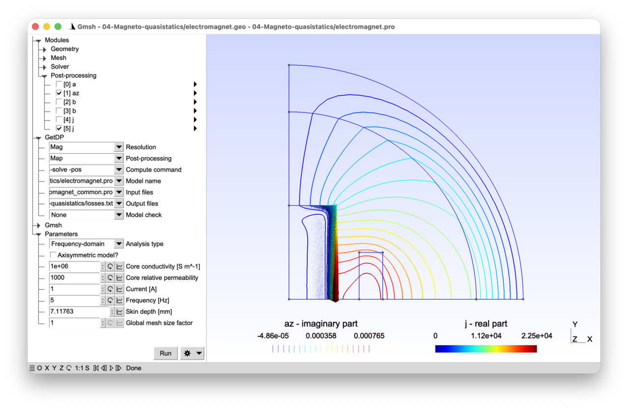
2.4 Tutorial 4: Magneto-quasistatic model of an electromagnet 
We consider the same electromagnet model as in tutorial 3, but in magneto-quasistatic regime, i.e. allowing for time-dependent currents in the inductor and eddy currents in the core. We still consider an imposed current density in the inductor, neglecting skin and proximity effects in the coil turns. In addition to the 2D model (invariant along the z-axis) we also consider an axisymmetric model (invariant by rotation around the y-axis).
2.4.1 Features 
- Magneto-quasistatic model in terms of the magnetic vector potential
- Axisymmetric model
- Time- and frequency-domain resolutions
- Post-processing of integral quantities
See the comments in electromagnet.pro and electromagnet.geo for details.
2.4.2 Running the tutorial 
On the command line:
> gmsh electromagnet.geo -2
> getdp electromagnet.pro -solve Mag -pos Map
Interactively with Gmsh: open electromagnet.pro with “File->Open”, then press “Run”.
2.4.3 Contents 
File electromagnet_common.pro 
// Parameters shared by Gmsh and GetDP.

mm = 1e-3;

dxCore = 50 * mm;
dyCore = 100 * mm;
xCoil = 75 * mm;
dxCoil = 25 * mm;
dyCoil = 100 * mm;
rInt = 200 * mm;
rExt = 250 * mm;
File electromagnet.geo 
// Gmsh script describing the geometry of the electromagnet. This is a pared
// down version of the geometry from tutorial 3, where all symmetries are
// taken advantage of.

Include "electromagnet_common.pro";

SetFactory("OpenCASCADE");
Rectangle(1) = {-dxCore, -dyCore, 0, 2 * dxCore, 2 * dyCore};
Rectangle(2) = {xCoil, -dyCoil / 2, 0, dxCoil, dyCoil};
Rectangle(3) = {-xCoil - dxCoil, -dyCoil / 2, 0, dxCoil, dyCoil};
Disk(4) = {0, 0, 0, rInt};
Disk(5) = {0, 0, 0, rExt};
d = 1.1 * rExt;
Rectangle(6) = {0, 0, 0, d, d};
BooleanIntersection{ Surface{6}; Delete; }{ Surface{1:5}; Delete; }

core() = Closest{0, 0, 0}{ Surface{:}; };
air() = Closest{dxCore + mm, 0, 0}{ Surface{:}; };
airinf() = Closest{rInt + mm, 0, 0}{ Surface{:}; };
indr() = Closest{xCoil + mm, 0, 0}{ Surface{:}; };
Physical Surface("Core", 1) = core(0);
Physical Surface("Air", 2) = air(0);
Physical Surface("AirInf", 3) = airinf(0);
Physical Surface("CoilRight", 4) = indr(0);

bot() = Curve In BoundingBox{-mm, -mm, -mm, d, mm, mm};
left() = Curve In BoundingBox{-mm, -mm, -mm, mm, d, mm};
inf() = CombinedBoundary{ Surface{:}; };
inf() -= {bot(), left()};
Physical Curve("Bottom", 10) = bot();
Physical Curve("Left", 11) = left();
Physical Curve("Inf", 12) = inf();

// Mesh size constraints:
DefineConstant[
  s = {1, Name "Parameters/}Global mesh size factor"}
];

MeshSize{:} = 12.5 * mm * s;
MeshSize{ PointsOf{ Surface{indr(0)}; } } = 5 * mm * s;
MeshSize{ PointsOf{ Surface{core(0)}; } } = 4 * mm * s;

// Refine to capture the skin depth:
skin() = Curve In BoundingBox{dxCore - mm, -mm, -mm, dxCore + mm, d, mm};
MeshSize{ PointsOf{ Curve{skin(0)}; } } = 0.5 * mm * s;
File electromagnet.pro 
// This model computes the magnetic field produced by an AC current in the same
// electromagnet as the one considered in tutorial 3 with a DC current.
//
// This corresponds to a magneto-quasistatic (or "magnetodynamic") physical
// model, obtained by combining the Maxwell-Ampere equation where the
// displacement current is neglected ("curl h = j", with "h" the magnetic field
// and "j" the current density), the Faraday equation ("curl e = -\partial_t b",
// with "e" the electric field and "b" the magnetic flux density), the magnetic
// Gauss law ("div b = 0"), the magnetic constitutive law ("b = mu h", with "mu"
// the magnetic permeability) and Ohm's law ("j = sigma e", with "sigma" the
// electric conductivity). In the coil of the electromagnet we assume that eddy
// currents can be neglected and we simply impose a source current density "j =
// js". This is a standard modeling choice for "stranded" coils made of many
// thin insulated wires: each wire is thin compared to the skin depth, which
// prevents eddy loops from forming inside the coil. The assumption would no
// longer be valid for a massive ("solid") conductor, or for a coil connected to
// a voltage source (see tutorial 7), potentially through a circuit (see
// tutorial 8).
//
// We can introduce a vector magnetic potential "a" such that "b = curl a"
// and "e = -\partial_t a", that satisfies both Gauss' law and Faraday's
// equation. We call this the "modified" vector potential because the usual
// definition "e = -\partial_t a - grad v" has been simplified by implicitly
// fixing the electric scalar potential "v" to zero -- equivalently, we have
// chosen a gauge that absorbs "grad v" into "a". This is a valid choice
// whenever the current is imposed (as here) rather than driven by a voltage.
// In tutorial 7 we will reintroduce "v" to allow prescribing a voltage drop
// or computing it from an imposed current, using the so-called "a-v"
// formulation.
//
// Plugging this vector potential into Ampere's equation and using the
// constitutive laws leads to
//
//   curl(nu curl a) + sigma \partial_t a = js
//
// where "nu = 1/mu" is the magnetic reluctivity. The right-hand side is the
// imposed (source) current density; on the left-hand side, "sigma \partial_t
// a" is the induced (eddy) current density, due to the time-varying magnetic
// flux. The total current density in a conducting region is thus
// "j = -sigma \partial_t a" (purely induced) and in a source region it is
// "j = js" (purely imposed). See the PostProcessing section below, which
// defines the full "j" piecewise on the two kinds of regions.
//
// We consider both time-domain (transient) and frequency-domain (steady-state)
// resolutions, with a sinusoidal source current density at fixed frequency f:
//
//   js(t) = (0, 0, Js sin(2 pi f t))
//
// As in tutorial 3, with a source current density along the z-axis, the
// magnetic vector potential a is a vector field with a single non-zero
// component along the z-axis, i.e.,
//
//   a(x, y, t) = (0, 0, az(x, y, t))
//
// and we can use the same "Form1P" function space with the same
// "BF_PerpendicularEdge" basis functions.
//
// In the time-domain an implicit Euler time stepping scheme is used, whereas in
// the frequency domain, we solve for the phasor "A(x, y)" such that
//
//   a(x, y, t) = Re( A(x, y) exp(i 2 pi f t) )
//
// Note that with this definition of phasors in terms of peak values, a factor
// 1/2 appears in time-averaged quadratic quantities such as electromagnetic
// power (due to the time-averaged cosine squared over a period). This factor
// dissapears for phasors defined in terms of RMS values, or for the calculation
// of instantaneous power in the time-domain.

Include "electromagnet_common.pro";

Group {
  // Physical regions:
  Core = Region[ 1 ];
  Air = Region[ 2 ];
  AirInf = Region[ 3 ];
  CoilRight = Region[ 4 ];
  Bottom = Region[ 10 ];
  Left = Region[ 11 ];
  Inf = Region[ 12 ];

  // Abstract regions:
  //  - "Vol_Mag": full volume domain
  //  - "Vol_S_Mag": region with imposed current source js
  //  - "Vol_C_Mag": conducting regions with eddy currents
  //  - "Vol_Inf_Mag": region with infinite ring geometric transformation
  //  - "Sur_Neu_Mag": part of the boundary with non-homogeneous Neumann
  //    conditions
  Vol_Mag     = Region[ {Air, AirInf, Core, CoilRight} ];
  Vol_S_Mag   = Region[ CoilRight ];
  Vol_C_Mag   = Region[ Core ];
  Vol_Inf_Mag = Region[ AirInf ];
  Sur_Neu_Mag = Region[ {} ]; // empty
}

Function {
  DefineConstant[
    AnalysisType = {1, Choices{0="Time-domain", 1="Frequency-domain"},
      Name "Parameters/Analysis type"}
    // In addition to a 2D model (invariant along the z-axis) we also consider
    // an axisymmetric model (invariant by rotation around the y-axis). This is
    // appropriate when the 3D device is itself a solid of revolution -- as with
    // a cylindrical coil. It would not be appropriate for, e.g., a
    // rotating-machine cross-section, which is only piecewise-invariant by
    // rotation:
    Axisymmetric = {0, Choices{0, 1},
      Name "Parameters/Axisymmetric model?"}
    Current = {1, Min 0.01, Max 100, Step 0.1,
      Name "Parameters/Current [A]"}
    f = {5, Min 1, Max 1000, Step 1,
      Name "Parameters/Frequency [Hz]"}
    mur = {1000, Min 1, Max 5000, Step 1,
      Name "Parameters/Core relative permeability"}
    sigma = {1e6, Min 1, Max 1e6, Step 100,
      Name "Parameters/Core conductivity [S m^-1]"}
  ];

  T = 1 / f;
  dt = T / 20;
  tmax = 2 * T;

  mu0 = 4.e-7 * Pi;
  nu0 = 1 / mu0;
  nu [ Region[{Air, AirInf, CoilRight}] ] = nu0;
  nu [ Core ]  = 1 / (mur * mu0);

  sigma[ Core ] = sigma;

  SkinDepth = DefineNumber[ 1e3 * Sqrt[2 / (2 * Pi * f * mur * mu0 * sigma)],
    Name "Parameters/Skin depth [mm]", ReadOnly];

  NbTurns = 1000;

  // The built-in function "F_Sin_wt_p[]{2 * Pi * f, 0}" will be interpreted as
  // "Sin[2 * Pi * f * $Time]" in the time domain, where "$Time" denotes the
  // current value of time, and as "Complex[0, -1]" in the frequency domain.
  //
  // The syntax "Complex[Re, Im]" builds a complex number from its real and
  // imaginary parts: "Complex[0, 1]" is the imaginary unit "i", and "Complex[0,
  // -1] = -i" is the phasor of "sin(omega t)" under the convention "x(t) = Re[X
  // exp(i omega t)]" (indeed, "sin(omega t) = Re[-i exp(i omega t)]").
  js[ CoilRight ] = Vector[0, 0, -NbTurns * Current / (dxCoil * dyCoil)] *
    F_Sin_wt_p[]{2 * Pi * f, 0};

  // Coefficient for computing electromagnetic power: 1 for time-domain
  // (instantaneous) power or for RMS phasors, 1/2 for peak-valued phasors:
  CoefPower = (AnalysisType == 0) ? 1 : 0.5;
}

Constraint {
  { Name a_Mag_2D;
    Case {
      { Region Left; Value 0.; }
      { Region Inf; Value 0.; }
    }
  }
}

Group {
  Dom_Hcurl_a_Mag_2D = Region[ {Vol_Mag, Sur_Neu_Mag} ];
}

FunctionSpace {
  { Name Hcurl_a_Mag_2D; Type Form1P;
    BasisFunction {
      { Name se; NameOfCoef ae; Function BF_PerpendicularEdge;
        Support Dom_Hcurl_a_Mag_2D; Entity NodesOf[ All ]; }
    }
    Constraint {
      { NameOfCoef ae; EntityType NodesOf; NameOfConstraint a_Mag_2D; }
    }
  }
}

Jacobian {
  { Name Vol;
    Case {
      // Solving an axisymmetric problem in GetDP is achieved by specifying the
      // axisymmetric variants of the Jacobian transformations, i.e. replacing
      // "Vol" with "VolAxi" and "VolSphShell" with "VolAxiSphShell":
      If(Axisymmetric)
        { Region Vol_Inf_Mag; Jacobian VolAxiSphShell {rInt, rExt}; }
        { Region All; Jacobian VolAxi; }
        // The axisymmetric Jacobians assume that the domain is in the z == 0
        // plane, and that the rotation axis is the y-axis.
      Else
        { Region Vol_Inf_Mag; Jacobian VolSphShell {rInt, rExt}; }
        { Region All; Jacobian Vol; }
      EndIf
    }
  }
}

Integration {
  { Name Int;
    Case {
      { Type Gauss;
        Case {
          // With pieceweise linear basis functions we must be able to integrate
          // quadratic polynomials in "Vol_C_Mag", hence we use 4 integration
          // points instead of 1 as in tutorial 3:
          { GeoElement Triangle; NumberOfPoints 3; }
        }
      }
    }
  }
}

// The weak formulation is derived in a similar way as for the magnetostatic
// problem from tutorial 3: find "a" such that
//
//   (curl(nu curl a), a')_Vol_Mag + (sigma \partial_t a, a')_Vol_C_Mag
//     = (js, a')_Vol_S_Mag
//
// holds for all test functions "a'". After integration by parts, and with the
// same boundary conditions as in tutorial 3, it reads: find a such that
//
//   (nu curl a, curl a')_Vol_Mag + (sigma \partial_t a, a')_Vol_C_Mag
//     = (js, a')_Vol_S_Mag
//
// holds for all test functions "a'".
Formulation {
  { Name Magnetoquasistatics_a_2D; Type FemEquation;
    Quantity {
      { Name a; Type Local; NameOfSpace Hcurl_a_Mag_2D; }
    }
    Equation {
      Integral { [ nu[] * Dof{d a} , {d a} ];
        In Vol_Mag; Jacobian Vol; Integration Int; }

      Integral { DtDof [ sigma[] * Dof{a} , {a} ];
        In Vol_C_Mag; Jacobian Vol; Integration Int; }

      Integral { [ - js[] , {a} ];
        In Vol_S_Mag; Jacobian Vol; Integration Int; }
    }
  }
}

Resolution {
  { Name Mag;
    System {
      { Name Sys_Mag; NameOfFormulation Magnetoquasistatics_a_2D;
        If(AnalysisType == 1)
          // With "Type Complex" and "Frequency f", GetDP transforms the "DtDof"
          // operator as a multiplication by "Complex[0, 2 * Pi * f]", and
          // handles all fields as complex-valued phasors:
          Type Complex; Frequency f;
        EndIf
      }
    }
    Operation {
      If(AnalysisType == 1)
        Generate[Sys_Mag]; Solve[Sys_Mag]; SaveSolution[Sys_Mag];
      Else
        // If no "Init" constraint is given, "InitSolution[]" initializes the
        // solution to 0:
        InitSolution[Sys_Mag];
        TimeLoopTheta[0, tmax, dt, 1] {
          Generate[Sys_Mag]; Solve[Sys_Mag]; SaveSolution[Sys_Mag];
        }
      EndIf
    }
  }
}

PostProcessing {
  { Name Mag; NameOfFormulation Magnetoquasistatics_a_2D;
    Quantity {
      { Name a;
        Value {
          Term { [ {a} ]; In Vol_Mag; Jacobian Vol; }
        }
      }
      { Name az; // z-component of the vector potential
        Value {
          Term { [ CompZ[{a}] ]; In Vol_Mag; Jacobian Vol; }
        }
      }
      { Name b;
        Value {
          Term { [ {d a} ]; In Vol_Mag; Jacobian Vol; }
        }
      }
      { Name h;
        Value {
          Term { [ nu[] * {d a} ]; In Vol_Mag; Jacobian Vol; }
        }
      }
      // The current density can be defined piecewise: as the induced (eddy)
      // current density in the conducting regions, and as the source current
      // density in the inductor regions:
      { Name j;
        Value {
          Term { [ - sigma[] * Dt[{a}] ]; In Vol_C_Mag; Jacobian Vol; }
          Term { [ js[] ]; In Vol_S_Mag; Jacobian Vol; }
        }
      }
      // We can compute Joule losses by integrating "1 / sigma |j|^2" over the
      // domain (beware of time-averaging with phasors, cf. the definition of
      // "CoefPower" above), which can be done by defining an "Integral"
      // post-processing quantity, again piecewise. In the conducting regions
      // the current is induced, "j = -sigma \partial_t a", so "|j|^2 / sigma =
      // sigma |\partial_t a|^2". In the source regions the current is imposed,
      // and we keep "|js|^2 / sigma" directly:
      { Name JouleLosses;
        Value {
          Integral { [ CoefPower * sigma[] * SquNorm[Dt[{a}]] ];
            In Vol_C_Mag; Jacobian Vol; Integration Int; }
          Integral { [ CoefPower / sigma[] * SquNorm[js[]] ];
            In Vol_S_Mag; Jacobian Vol; Integration Int; }
        }
      }
    }
  }
}

PostOperation {
  { Name Map; NameOfPostProcessing Mag;
    Operation {
      // In the time domain, the output files will contain the values at each
      // time step. In the frequency domain, they will contain two values: the
      // real and imaginary parts.
      Print[ a, OnElementsOf Vol_Mag, File "a.pos" ];
      Print[ az, OnElementsOf Vol_Mag, File "az.pos" ];
      Print[ b, OnElementsOf Vol_Mag, File "b.pos" ];
      Print[ b, OnLine{{mm, mm, 0}{rInt, mm, 0}}{50}, File "cutb.pos" ];
      Print[ j, OnElementsOf Vol_S_Mag, File "js.pos" ];
      Print[ j, OnElementsOf Vol_C_Mag, File "j.pos" ];
      // Integral post-processing quantities do not make sense on elements on
      // the mesh, as they are global values. Here we evaluate the Joule losses
      // over the conducting regions:
      Print[ JouleLosses[Vol_C_Mag], OnGlobal, Format Table, File "losses.txt" ];
    }
  }
}
2.5 Tutorial 5: Full-wave model of a rectangular waveguide 
A full-wave time-harmonic Maxwell model of a rectangular waveguide is considered, in both 2D and 3D. The electric field is discretized with edge elements, with perfectly electrically conducting (PEC) walls, a Silver-Muller absorbing boundary condition on the outer domain boundary, and a modal excitation imposed at the input port through an auxiliary projection resolution.
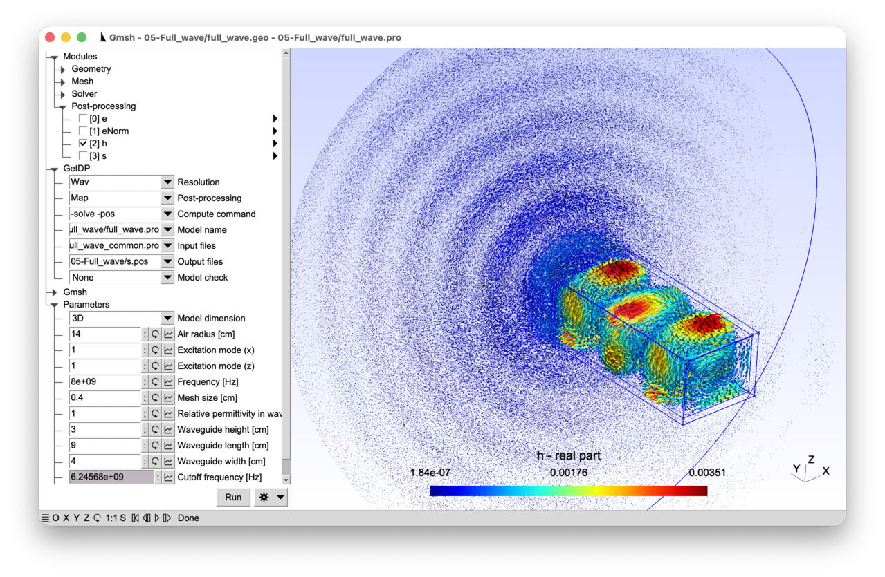
2.5.1 Features 
- Harmonic full-wave Maxwell formulation in terms of the electric field
- Edge finite elements (lowest-order Whitney elements in H(curl))
- Two- and three-dimensional models
- Dirichlet boundary condition through an auxiliary resolution
See the comments in full_wave.pro and full_wave.geo for details.
2.5.2 Running the tutorial 
On the command line (2D analysis):
> gmsh full_wave.geo -2
> getdp full_wave.pro -solve Wav -pos Map
On the command line (3D analysis):
> gmsh full_wave.geo -3 -setnumber dim 3
> getdp full_wave.pro -solve Wav -pos Map -setnumber dim 3
Interactively with Gmsh: open full_wave.pro with “File->Open”, then press “Run”.
2.5.3 Contents 
File full_wave_common.pro 
DefineConstant[
  dim = {2, Choices{2="2D", 3="3D"},
    Name "Parameters/0Model dimension"}
  Wx = {4, Min 1, Max 100, Step 1,
    Name "Parameters/Waveguide width [cm]"}
  Wz = {3, Min 1, Max 100, Step 1, Visible (dim == 3),
    Name "Parameters/Waveguide height [cm]"}
];

// back to meters:
Wx = Wx / 100;
Wz = Wz / 100;
File full_wave.geo 
SetFactory("OpenCASCADE");

Include "full_wave_common.pro";

DefineConstant[
  L = {9, Min 1, Max 100, Step 1,
    Name "Parameters/Waveguide length [cm]"}
  res = {0.4, Min 1e-2, Max 50e-1, Step 1e-2,
    Name "Parameters/Mesh size [cm]"}
  airRadius = {6, Min 0, Max 100, Step 1,
    Name "Parameters/Air radius [cm]"}
];

// Convert dimensions back to meters:
L = L / 100;
res = res / 100;
airRadius = airRadius / 100;

// Inner part of waveguide:
xMinIn = -Wx / 2;
yMinIn = -L;
zMinIn = -Wz / 2;

// Wall thickness:
t = 2e-3;

// Outer part of waveguide:
xMinOut = xMinIn - t;
yMinOut = yMinIn - t;
zMinOut = zMinIn - t;
WxOut = Wx + 2 * t;
WzOut = Wz + 2 * t;

If(dim == 2)
  // 2D geometry in z == 0 plane:
  zMinIn = 0;
  zMinOut = 0;
  If(airRadius > 0)
    Disk(1) = {0, 0, 0, airRadius};
    Rectangle(2) = {xMinOut, yMinOut, zMinOut, WxOut, L + t};
    vAir() = BooleanDifference{ Surface{1}; Delete; }{ Surface{2}; Delete; };
  Else
    vAir() = {};
  EndIf
  vGuideIn = news; // next available surface tag
  Rectangle(vGuideIn) = {xMinIn, yMinIn, zMinIn, Wx, L};
Else
  // 3D geometry:
  If(airRadius > 0)
    Sphere(1) = {0, 0, 0, airRadius};
    Box(2) = {xMinOut, yMinOut, zMinOut, WxOut, L + t, WzOut};
    vAir() = BooleanDifference{ Volume{1}; Delete; }{ Volume{2}; Delete; };
  Else
    vAir() = {};
  EndIf
  vGuideIn = newv; // next available volume tag
  Box(vGuideIn) = {xMinIn, yMinIn, zMinIn, Wx, L, Wz};
EndIf

If(airRadius > 0)
  // Make all entities conformal (see tutorial 3):
  Coherence;
EndIf

// Retrieve surfaces for boundary conditions using a bounding box search, with a
// small tolerance:
tol = 1e-6;

// Excitation port at yMinIn:
sPort() = GeoEntity{dim - 1} In BoundingBox {
  xMinIn - tol, yMinIn - tol, zMinIn - tol,
  xMinIn + Wx + tol, yMinIn + tol, zMinIn + Wz + tol};

// Output port at yMinIn + L:
sOut() = GeoEntity{dim - 1} In BoundingBox {
  xMinIn - tol, yMinIn + L - tol, zMinIn - tol,
  xMinIn + Wx + tol, yMinIn + L + tol, zMinIn + Wz + tol};

// Waveguide walls excluding ports for PEC conditions:
sPEC() = GeoEntity{dim - 1} In BoundingBox {
  xMinOut - tol, yMinOut - tol, zMinOut - tol,
  xMinOut + WxOut + tol, yMinOut + L + t + tol, zMinOut + WzOut + tol};
sPEC() -= {sPort(), sOut()};

// Infinite boundary for ABC. "CombinedBoundary" returns the exterior boundary
// curves (resp. surfaces) of a set of surfaces (resp. volumes), combining
// (i.e. removing) internal boundaries shared by adjacent entities.  Here it
// returns the outermost boundary of the entire model:
sInf() = CombinedBoundary{ GeoEntity{dim}{:}; };
sInf() -= {sPort(), sOut(), sPEC()};

// Uniform mesh size constraint:
MeshSize{:} = res;

// Physical groups:
Physical GeoEntity{dim}("Waveguide", 1000) = {vGuideIn};
Physical GeoEntity{dim}("Air", 1001) = {vAir()};
Physical GeoEntity{dim - 1}("PEC", 2000) = {sPEC()};
Physical GeoEntity{dim - 1}("Port", 2001) = {sPort()};
Physical GeoEntity{dim - 1}("Inf", 2002) = {sInf()};
File full_wave.pro 
// In this tutorial we introduce the full-wave Maxwell problem in the frequency
// domain, with lowest order Whitney edge elements to discretize the vector
// electric field in both 2D and 3D. The vector-valued basis functions are
// associated with the edges of the mesh, i.e. the electric field "e(x, y, z)"
// is expanded as
//
//   e(x, y, z) = Sum_{k in E} ee_k se_k(x, y, z)
//
// where the sum runs over all the edges of the mesh and the vector-valued edge
// basis functions "se_k(x, y, z)" are tangentially continuous across the mesh
// elements. The coefficients "ee_k" (i.e. the values of the degrees of
// freedom), correspond to the circulations of the electric field on the edges
// of the mesh. This identification between DoFs and edge circulations is a
// defining property of the lowest-order Whitney edge element: each basis
// function "se_k" is designed so that its line integral along edge "k" is
// equal to 1, and its line integral along any other edge is equal to 0. By
// linearity, "\int_{edge k} e . dl = ee_k", so each coefficient "ee_k" is
// literally the circulation of "e" along edge "k".
//
// Edge elements are one member of a larger family known as Whitney
// elements. Nodal "BF_Node" functions (associated with nodes, one pointwise
// scalar DoF per node) discretize scalar field and belong to "H1"; edge
// "BF_Edge" functions (associated with edges, one circulation DoF per edge)
// discretize vector fields whose curl must remain square-integrable and belong
// to "H(curl)"; facet "BF_Facet" functions (associated with faces, one flux DoF
// per face) discretize vector fields whose divergence must remain
// square-integrable and belong to "H(div)"; and volume "BF_Volume" functions
// (associated with elements, one DoF per element) discretize scalar densities
// in "L2". These spaces are linked by the gradient, curl and divergence
// operators: "grad" maps "H1" into "H(curl)", "curl" maps "H(curl)" into
// "H(div)", and "div" maps "H(div)" into "L2", reflecting the identities "curl
// grad = 0" and "div curl = 0" at the discrete level.  Each physical quantity
// in encountered in the tutorials has a natural home in this hierarchy: "v" and
// "T" live in "H1", "e" and "h" live in "H(curl)", "b" and "d" live in
// "H(div)", and charge or energy densities live in "L2".
//
// We model a rectangular waveguide, excited by a given electric field mode on
// an input port. Since the degrees of freedom correspond to the circulation of
// the electric field, imposing a Dirichlet boundary condition is not as trivial
// as with Lagrange finite elements (where the coefficients correspond to the
// value of the field at the nodes). With edge elements, the coefficients will
// change depending on the length and the orientation of the mesh edges: in this
// tutorial we will use a pre-resolution to compute the coefficients on the
// waveguide port.
//
// We assume that the waveguide is a good conductor, so we impose a "Perfect
// Electric Conductor" (PEC) boundary condition on the rest of the waveguide
// boundary, which amounts to imposing that the tangential component of the
// electric field, "e_t", is zero. Since the degrees of freedom are the
// circulation of the electric field, this amounts to setting the coefficients
// "ee_k" to 0 on the boundary edges of the waveguide.
//
// To truncate the computational domain, we cannot use the same infinite
// elements as in tutorial 3: the oscillatory nature of the wave solution
// prevents simply compressing an outside ring around the computational
// domain. Instead, we use a Silver-Muller Absorbing Boundary Condition (ABC),
// which expresses that the field behaves locally like an outgoing plane wave:
//
//   n x h = - sqrt(epsilon / mu) e_t,
//
// with "n" the exterior normal on the boundary, "h" the magnetic field,
// "epsilon" the dielectric permittivity, "mu" the magnetic permeability and
// "e_t = e - (e . n) n = (n x e) x n" the tangential electric field.
//
// We use the same phasor convention as in tutorial 4, i.e. "e(x, y, z, t) = Re(
// E(x, y, z) exp(i omega t) )", with the angular frequency "omega = 2 pi f".

Group {
  // Physical regions:
  Waveguide = Region[ 1000 ];
  Air = Region[ 1001 ];
  BndPEC = Region[ 2000 ]; // Boundary with PEC condition
  BndPort = Region[ 2001 ]; // Input port
  BndInf = Region[ 2002 ]; // Boundary with ABC

  // Abstract regions:
  //  - "Vol_Wav": overall domain
  //  - "Sur_Port_Wav": port with imposed electric field mode
  //  - "Sur_Inf_Wav": truncation surface with absorbing boundary condition
  Vol_Wav = Region[ {Waveguide, Air} ];
  Sur_Port_Wav = Region[ BndPort ];
  Sur_Inf_Wav = Region[ BndInf ];
}

Include "full_wave_common.pro";

Function {
  eps0 = 8.8541878176e-12;
  mu0 = 4 * Pi * 1e-7;

  DefineConstant[
    m = { 1, Min 1, Max 10, Step 1,
      Name "Parameters/Excitation mode (x)"},
    n = { 1, Min 1, Max 10, Step 1, Visible (dim == 3),
      Name "Parameters/Excitation mode (z)"},
    epsr = { 1, Min 1, Max 10, Step 0.1,
      Name "Parameters/Relative permittivity in waveguide"},
    f = { 8e9, Min 1e8, Max 1e10, Step 1e8,
      Name "Parameters/Frequency [Hz]"}
  ];

  epsilon[ Region[ {Air, BndInf} ] ] = eps0;
  epsilon[ Region[ {Waveguide, BndPort} ] ] = epsr * eps0;
  mu[] = mu0;
  nu[] = 1 / mu0;

  i[] = Complex[0, 1];
  omega = 2 * Pi * f;

  // The expressions that follow give the transverse electric-field profile of
  // the mode excited at the port, "ePort". Both in 2D and in 3D we excite a TM
  // mode (transverse magnetic with respect to the propagation direction y,
  // i.e. "H_y = 0"). In a TM mode, all six field components can be recovered
  // from the single longitudinal scalar "E_y" by algebra and one transverse
  // derivative (see the explicit formulas below).
  //
  // In our FEM setup we do not impose "E_y" at the port: only the tangential
  // components -- "E_x" in 2D, and "(E_x, E_z)" in 3D -- are prescribed there,
  // and "E_y" emerges in the interior as part of the full vector solve. The "0"
  // written for the y-component of "ePort" below is normal to the port and is
  // silently dropped by the tangential L2 projection on "Sur_Port_Wav".
  //
  // The generating scalar "E_y" satisfies a Helmholtz equation with Dirichlet
  // BC at the PEC walls ("E_y" being tangential to them):
  //   - In 3D,
  //
  //         E_y = E_0 sin(kx (x - Wx / 2)) sin(kz (z - Wz / 2)),
  //
  //     giving the TM_mn mode of the rectangular waveguide. Both indices must
  //     satisfy "m >= 1" and "n >= 1", otherwise "E_y" vanishes identically and
  //     the mode degenerates (the family TM_m0 or TM_0n does not exist).
  //   - In 2D the geometry is invariant in z (no PEC walls at z = const), so
  //     only "kx = m Pi / Wx" is quantized:
  //
  //        E_y = E_0 sin(kx (x - Wx / 2)),
  //
  //     giving the TM_m mode of the parallel-plate waveguide (m >= 1; the m = 0
  //     case would be the TEM mode).
  //
  // The transverse components follow from
  //
  //   E_x = -gamma / kc^2 * \partial_x E_y
  //
  // and (in 3D)
  //
  //   E_z = -gamma / kc^2 * \partial_z E_y,
  //
  // with "gamma" the longitudinal propagation constant and "kc^2 = kx^2 + kz^2"
  // in 3D, reducing to "kc^2 = kx^2" in 2D. From the dispersion relation
  //
  //   k^2 = kx^2 + kz^2 + (-i gamma)^2
  //
  // with "k = omega sqrt(mu eps)", it follows that
  //
  //   gamma = sqrt(k^2 - (kx^2 + kz^2)) * i
  //
  // i.e. "gamma" is purely imaginary above cutoff (propagating mode) and purely
  // real below cutoff (evanescent mode).

  k[] = omega * Sqrt[epsilon[] * mu[]];
  kx = m * Pi / Wx; // transverse wavevector (x)
  kz = n * Pi / Wz; // transverse wavevector (z)
  If(dim == 2)
    gamma[] = Sqrt[k[]^2 - kx^2] * i[];
    ePort[] = Vector[-gamma[] / kx * Cos[kx * (X[] - Wx / 2)], 0, 0];
  Else
    kc = Sqrt[kx^2 + kz^2];
    gamma[] = Sqrt[k[]^2 - kc^2] * i[];
    ePort[] = Vector[
      -gamma[] * kx / kc^2 * Cos[kx * (X[] - Wx / 2)] * Sin[kz * (Z[] - Wz / 2)],
      0.,
      -gamma[] * kz / kc^2 * Sin[kx * (X[] - Wx / 2)] * Cos[kz * (Z[] - Wz / 2)]
    ];
  EndIf

  c = 1 / Sqrt[epsr * eps0 * mu0];
  DefineConstant[
    lambda = {c / f * 100, ReadOnly 1, Highlight "LightGrey",
      Name "Parameters/}Wavelength [cm]"},
    f_cutoff = { (dim == 2) ? (0.5 * c * m / Wx) :
      0.5 * c * Sqrt[(m * m) / (Wx * Wx) + (n * n) / (Wz * Wz)],
      ReadOnly 1, Highlight "LightGrey",
      Name "Parameters/}Cutoff frequency [Hz]"}
  ];
}

Jacobian {
  // Instead of explicitly defining a Jacobian method for volumes and surfaces,
  // a single Jacobian method can be defined piecewise:
  { Name Jac;
    Case {
      { Region Sur_Port_Wav; Jacobian Sur; }
      { Region Sur_Inf_Wav; Jacobian Sur; }
      { Region Vol_Wav; Jacobian Vol; }
    }
  }
}

Integration {
  { Name Int;
    Case {
      { Type Gauss;
        Case {
          { GeoElement Line; NumberOfPoints 4; }
          { GeoElement Triangle; NumberOfPoints 4; }
          { GeoElement Tetrahedron; NumberOfPoints 4; }
        }
      }
    }
  }
}

Constraint {
  { Name e_Wav;
    Case {
      // On the PEC boundary, the circulation of the electric field is imposed
      // to 0 on the edges:
      { Region BndPEC; Type Assign; Value 0.; }
      // On the input port, the circulation of the electric field is imposed
      // through the resolution of a linear system, performing the L2 projection
      // of a known mode:
      { Region BndPort; Type AssignFromResolution; NameOfResolution Proj_e; }
    }
  }
}

Group{
  Dom_Hcurl_e_Wav =  Region[ {Vol_Wav, Sur_Port_Wav, Sur_Inf_Wav} ];
}

FunctionSpace {
  // The electric "e" field belongs to H(curl), meaning that both "e" and "curl
  // e" are square integrable. Basis functions "BF_Edge" are associated with the
  // edges of the mesh, and ensure the tangential continuity of the electric
  // field across mesh elements:
  { Name Hcurl_e_Wav; Type Form1;
    BasisFunction {
      { Name se; NameOfCoef ee; Function BF_Edge;
        Support Dom_Hcurl_e_Wav; Entity EdgesOf[All]; }
    }
    Constraint {
      { NameOfCoef ee; EntityType EdgesOf; NameOfConstraint e_Wav; }
    }
  }
}

Formulation {
  // To derive the finite element formulation in terms of the electric field e
  // in the frequency domain, we start from Faraday's law:
  //
  //   curl e = - i omega b,
  //
  // with "b = mu h" the magnetic flux density. Taking its curl and introducing
  // the reluctivity "nu = 1 / mu", we get
  //
  //   curl (nu curl e) = -i omega curl h.
  //
  // Assuming no conduction currents (we treat the waveguide walls as perfect
  // conductors), Maxwell-Ampere's equation reduces to
  //
  //   curl h = i omega d,
  //
  // with "d = epsilon e" the displacement field. Combining the last two
  // equations leads to the strong form
  //
  //   curl (nu curl e) - omega^2 epsilon e = 0.
  //
  // The weak formulation is obtained by multiplying by test functions "e'" in
  // H(curl) and integrating over the domain "Vol_Wav". This leads to finding
  // "e" such that
  //
  //   (curl (nu curl e), e')_Vol_Wav - (omega^2 epsilon e, e')_Vol_Wav = 0.
  //
  // holds for all test functions "e'". After integration by parts, the weak form
  // becomes: find e such that, for all "e'":
  //
  //   (nu curl e, curl e')_Vol_Wav + (n x nu curl e, e')_Bnd_Vol_Wav
  //      - (omega^2 epsilon e, e')_Vol_Wav = 0.
  //
  // The boundary term vanishes where Dirichlet boundary conditions are applied
  // (PEC and input port). On the outside boundary, the Silver-Muller ABC leads
  // to a Robin boundary condition:
  //
  //   (n x nu curl e, e')_Sur_Inf
  //     = (n x nu (- i omega b), e')_Sur_Inf
  //     = - (i omega n x h, e')_Sur_Inf
  //     = (i omega sqrt(epsilon / mu) e_t, e')_Sur_Inf
  //
  { Name FullWave_e; Type FemEquation;
    Quantity {
      { Name e; Type Local; NameOfSpace Hcurl_e_Wav; }
    }
    Equation {
      Integral { [ nu[] * Dof{d e} , {d e} ];
        In Vol_Wav; Integration Int; Jacobian Jac; }

      Integral { [ -omega^2 * epsilon[] * Dof{e} , {e} ];
        In Vol_Wav; Integration Int; Jacobian Jac; }

      Integral { [ i[] * omega * Sqrt[epsilon[] / mu[]] * Dof{e} , {e} ];
        In Sur_Inf_Wav; Integration Int; Jacobian Jac; }
    }
  }

  // In order to compute the coefficients of the imposed electric field mode on
  // the input port, we define an auxiliary weak formulation to perform the
  // L2-projection of the "ePort[]" function onto the finite element basis: find
  // "e" such that
  //
  //   (e, e')_Sur_Port_Wav - (ePort, e')_Sur_Port_Wav = 0
  //
  // holds for all test functions "e'".
  //
  // A direct Dirichlet assignment (as we did for the PEC boundary above, where
  // the imposed circulation was simply zero) is impractical here: each
  // coefficient "ee_k" is an integral of "ePort" along an individual mesh edge,
  // which would have to be computed by hand for every edge on the port --
  // depending on its length, orientation, and the local value of "ePort".  The
  // L2 projection does this automatically and consistently: it solves a small
  // auxiliary system whose solution is, by construction, the best
  // tangentially-continuous edge-element approximation of "ePort" on the port.
  { Name Projection_e; Type FemEquation;
    Quantity {
      { Name e; Type Local; NameOfSpace Hcurl_e_Wav; }
    }
    Equation {
      Integral { [ Dof{e} , {e} ];
        In Sur_Port_Wav; Integration Int; Jacobian Jac; }
      Integral { [ -ePort[] , {e} ];
        In Sur_Port_Wav; Integration Int; Jacobian Jac; }
    }
  }
}

Resolution {
  { Name Wav;
    System {
      { Name Sys_Wav; NameOfFormulation FullWave_e; Type Complex; }
    }
    Operation {
      Generate[Sys_Wav]; Solve[Sys_Wav]; SaveSolution[Sys_Wav];
    }
  }

  // One constraint associated to the function space used in the "FullWave_e"
  // formulation is of type "AssignFromResolution Proj_e". GetDP will
  // automatically perform the "Proj_e" resolution during the pre-processing
  // stage of the main "Wav" resolution:
  { Name Proj_e;
    System {
      { Name Sys_Proj; NameOfFormulation Projection_e; Type Complex;
        DestinationSystem Sys_Wav; }
    }
    Operation {
      // Note the "TransferSolution[]" operation, which will copy the ee_k
      // coefficients computed on "Sur_Port_Wav" into the "DestinationSystem"
      // "Sys_Wav", defined in the "Wav" resolution:
      Generate[Sys_Proj]; Solve[Sys_Proj]; TransferSolution[Sys_Proj];
    }
  }
}

PostProcessing {
  { Name Wav; NameOfFormulation FullWave_e;
    Quantity {
      { Name e;
        Value {
          Term{ [ {e} ]; In Vol_Wav; Jacobian Jac; }
        }
      }
      { Name eNorm;
        Value {
          Term{ [ Norm[{e}] ]; In Vol_Wav; Jacobian Jac; }
        }
      }
      { Name h;
        Value{
          Term{ [ i[] * nu[] / omega * {d e} ]; In Vol_Wav; Jacobian Jac; }
        }
      }
      // The (complex) Poynting vector "s = e x h*" gives the time-averaged
      // power flux density (with factor 1/2 for peak-value phasors). The symbol
      // "/\" is GetDP's cross-product operator; "Conj[...]" takes the complex
      // conjugate:
      { Name s;
        Value{
          Term{ [ 0.5 * {e} /\ Conj[i[] * nu[] / omega * {d e}] ]; In Vol_Wav;
            Jacobian Jac; }
        }
      }
    }
  }
}

PostOperation {
  { Name Map; NameOfPostProcessing Wav;
    Operation {
      Print [ e, OnElementsOf Vol_Wav, File "e.pos"];
      Print [ eNorm, OnElementsOf Vol_Wav, File "eNorm.pos"];
      Print [ h, OnElementsOf Vol_Wav, File "h.pos"];
      Print [ s, OnElementsOf Vol_Wav, File "s.pos"];
    }
  }
}
2.6 Tutorial 6: Global quantities in electrostatics 
We consider the same model as in tutorial 1, i.e. a 2D electrostatic model of a microstrip line with only one half of the geometry modelled by symmetry. We introduce global quantities (voltage and charge) in the function space, which allows to naturally handle floating potentials and to compute the capacitance.
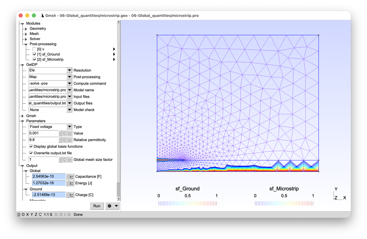
2.6.1 Features 
- Global quantities and their special basis functions
- Handling the floating potential and its energy dual, the charge
- Calculation of capacitances
- Fine-tuning of post-processing options
See the comments in microstrip.pro and microstrip.geo for details.
2.6.2 Running the tutorial 
On the command line:
> gmsh microstrip.geo -2
> getdp microstrip.pro -solve Ele -pos Map
Interactively with Gmsh: open microstrip.pro with “File->Open”, then press “Run”.
2.6.3 Contents 
File microstrip.geo 
// Gmsh script describing the geometry of the microstrip line and the associated
// meshing constraints.

// Dimensions (there are no units in Gmsh -- the following values should be
// interpreted as dimensions in meters due to the definition of the physical
// parameters in MKS units in "microstrip.pro"):
h = 1.e-3; // thickness of dielectric substrate
w = 4.72e-3; // width of microstrip line
t = 0.035e-3; // thickness of microstrip line
xBox = w/2. * 6.; // width of air box
yBox = h * 12.; // height of air box

// Global mesh size factor (that can be modified interactively in the Gmsh
// graphical interface):
s = DefineNumber[1., Name "Parameters/Global mesh size factor"];

// Target mesh sizes:
p0 = h / 10 * s;
pLine0 = w / 20 * s;
pLine1 = w / 100 * s;
pxBox = xBox / 10 * s;
pyBox = yBox / 8 * s;

// We create this first geometry in a bottom-up manner with the built-in Gmsh
// CAD kernel, successively defining model points, lines, loops and surfaces:
Point(1) = {0, 0, 0, p0};
Point(2) = {xBox, 0, 0, pxBox};
Point(3) = {xBox, h, 0, pxBox};
Point(4) = {0, h, 0, pLine0};
Point(5) = {w/2, h, 0, pLine1};
Point(6) = {0, h+t, 0, pLine0};
Point(7) = {w/2, h+t, 0, pLine1};
Point(8) = {0, yBox, 0, pyBox};
Point(9) = {xBox, yBox, 0, pyBox};
Line(1) = {1, 2};
Line(2) = {2, 3};
Line(3) = {3, 9};
Line(4) = {9, 8};
Line(5) = {8, 6};
Line(7) = {4, 1};
Line(8) = {5, 3};
Line(9) = {4, 5};
Line(10) = {6, 7};
Line(11) = {5, 7};
Curve Loop(12) = {1, 2, -8, -9, 7};
Plane Surface(13) = {12};
Curve Loop(14) = {10, -11, 8, 3, 4, 5};
Plane Surface(15) = {14};

// The last step is to define physical groups, assigning unique tags (and names)
// to groups of model entities. Physical groups serve two purposes: when they
// are defined they tell Gmsh which elements to save in the mesh file (by
// default only elements belonging to at least one physical group are saved),
// and they provide the tags that GetDP uses in "Region[]" to identify parts of
// the domain.
Physical Surface("Air", 1) = {15};
Physical Surface("Dielectric", 2) = {13};
Physical Curve("Ground", 10) = {1};
Physical Curve("Microstrip boundary", 11) = {9, 10, 11};
Physical Curve("Inf", 12) = {2, 3, 4};
File microstrip.pro 
// In a two-dimensional electrostatic model (see tutorial 1), the finite element
// expansion of the electric scalar potential "v(x, y)" associates basis
// functions with individual nodes in the mesh:
//
//   v(x, y) = Sum_{k in N} vn_k sn_k(x, y)
//
// with "N" the set of all the nodes in the mesh and "sn_k(x, y)" the Lagrange
// basis function associated with node "k". Now consider the situation where
// "v(x, y)" is constant over a region of the problem, e.g. "v(x, y) =
// vf_electrode" on an electrode. By factorizing the identical nodal values
// "vf_electrode", a global (non-local) basis function "sf_electrode(x, y)" is
// obtained as factor:
//
//   v(x, y) = Sum_{k in N} vn_k sn_k(x, y)
//     = Sum_{k in N \ E} vn_k sn_k(x, y) + Sum_{k in E} vn_k sn_k(x, y)
//     = Sum_{k in N \ E} vn_k sn_k(x, y) + vf_electrode Sum_{k in E} sn_k(x, y)
//     = Sum_{k in N \ E} vn_k sn_k(x, y) + vf_electrode sf_electrode(x, y)
//
// with "E" the set of nodes on the electrode. The global basis function
//
//   sf_electrode(x, y) = Sum_{k in E} sn_k(x, y)
//
// is the sum of the Lagrange (nodal) basis functions associated with the nodes
// of the electrode. This function
//  - is a continuous fonction, scalar in this case;
//  - is equal to 1 at the nodes of the electrode, and to 0 at all other nodes;
//  - decreases from 1 to 0 over the one-element-thick layer of elements sharing
//    at least one node with the electrode region.
//
// One such global basis function can be associated with each electrode in the
// system, so that the finite element expansion of the electric scalar potential
// reads:
//
//   v(x, y) = Sum_k vn_k sn_k(x, y)
//     + Sum_electrode vf_electrode sf_electrode(x, y)
//
// where "Sum_electrode" runs over all the electrodes in the model (one term per
// electrode, so two in the present example: the boundary of the microstrip line
// and the ground), and "Sum_k" runs over all nodes except those of the
// electrode regions.
//
// In this tutorial we modify the electrostatic problem from tutorial 1 to show
// how GetDP takes advantage of global basis functions
//  - to efficiently compute the electrode charges "Q_electrode", which are the
//    energy duals of the global "vf_electrode" potentials;
//  - to deal with floating potentials, which are the computed electrode
//    potentials when the electrode charge is imposed;
//  - to provide output global quantities (charges, voltages, capacitances) that
//    can be used in an external circuit.

Group {
  // Physical regions:
  Air = Region[ 1 ];
  Dielectric = Region[ 2 ];
  Ground = Region[ 10 ];
  Microstrip = Region[ 11 ];
  Inf = Region[ 12 ];

  // Abstract regions:
  //  - "Vol_Ele": overall domain
  //  - "Sur_Neu_Ele": surface with non homogeneous Neumann boundary conditions
  //  - "Sur_Electrodes_Ele": electrode regions
  Vol_Ele = Region[ {Air, Dielectric} ];
  Sur_Neu_Ele = Region[ {} ];
  Sur_Electrodes_Ele = Region [ {Ground, Microstrip} ];
}

Function {
  DefineConstant[
    TypeBC = {0, Choices{0="Fixed voltage", 1="Fixed charge"},
      Name "Parameters/0Type"}
    ValueBC = {1e-3,
      Name "Parameters/1Value"}
    epsr = {9.8,
      Name "Parameters/2Relative permittivity"}
    DisplayGlobalBasisFunctions = {0, Choices {0, 1},
      Name "Parameters/3Display global basis functions"}
    OverwriteOutput = {1, Choices {0, 1},
      Name "Parameters/4Overwrite output.txt file"}
  ];

  eps0 = 8.854187818e-12;
  epsilon[ Air ] = eps0;
  epsilon[ Dielectric ] = epsr * eps0;
}

Constraint {
  // The Dirichlet boundary condition on the local electric potential is only
  // used for the homogeneous condition on the top and right boundaries. The
  // boundary of the microstrip line and the ground are now treated as
  // electrodes, on which either the potential or the charge is imposed through
  // the "Voltage_Ele" or "Charge_Ele" constraints below.
  { Name v_Ele;
    Case {
      { Region Inf; Value 0; }
    }
  }

  { Name Voltage_Ele;
    Case {
      // If the "Fixed voltage" option is enabled (i.e. when "TypeBC == 0"),
      // impose the global potential on the boundary of the microstrip line (and
      // thus the voltage, i.e. the potential difference between the microstrip
      // and the ground) to "ValueBC":
      If(TypeBC == 0)
        { Region Microstrip; Value ValueBC; }
      EndIf
      // Impose the global (i.e. region-wise) potential to 0 on the ground
      // electrode:
      { Region Ground; Value 0; }
    }
  }
  { Name Charge_Ele;
    Case {
      // If the "Fixed charge" option is enabled (i.e. when "TypeBC == 1"),
      // impose the global charge on the boudary of the microstrip line:
      If(TypeBC == 1)
        { Region Microstrip; Value ValueBC; }
      EndIf
      // Since "Ground" is always constrained to zero potential by "Voltage_Ele"
      // above, its charge cannot be prescribed; it will be computed as a global
      // output, cf. "Q" in the PostProcessing below.
    }
  }
}

Group{
  Dom_H1_v_Ele =  Region[ {Vol_Ele, Sur_Neu_Ele, Sur_Electrodes_Ele} ];
}

FunctionSpace {
  // The natural treatment of global quantities in GetDP stems from the fact
  // that nearly all the work is done at the level of the FunctionSpace
  // definition. As seen above, the finite element expansion of the potential
  // "v" is
  //
  //   v(x, y) = Sum_k vn_k sn_k(x, y)
  //     + Sum_electrode vf_electrode sf_electrode(x, y)
  //
  // with "Sum_k" running over all nodes except those of the electrode
  // regions. The global basis function "sf_electrode(x, y)" is the sum of the
  // nodal basis functions associated with the nodes of the electrode. This is
  // precisely what one finds in the FunctionSpace definition below, where:
  //  - "BF_Node" is the standard Lagrange basis function, that we associate
  //    with all the nodes of the domain except those on the electrode regions
  //    ("Entity NodesOf[ All, Not Sur_Electrodes_Ele ]"). One degree of freedom
  //    is created per node of the region.
  //  - "BF_GroupOfNodes" is the sum of Lagrange basis functions associated with
  //    the group of nodes of the electrodes ("Entity GroupsOfNodesOf[
  //    Sur_Electrodes_Ele ]"). A single degree of freedom is shared by all the
  //    nodes of each listed region -- whose value is the "vf_electrode"
  //    coefficient attached to the global basis function "sf_electrode".
  //
  // By activating the "Display global basis functions" option, you can
  // visualize the two "sf_electrode" basis functions in the model: one
  // associated with the boundary of the microstrip line, the other with the
  // ground.
  //
  // The global quantities are attributed an explicit name in the
  // "GlobalQuantity" section; these names are used in the corresponding
  // "GlobalTerm" in the Formulation. Such global terms are the equivalent of a
  // "Integral" term, but where no integration needs to be performed. The
  // "AssociatedWith" statement refers to the fact that the global potential of
  // an electrode is the (electrostatic) energy dual of the electric charge
  // carried by that electrode. Indeed, let us consider the electrostatic weak
  // formulation derived in tutorial 1: find "v" in H1_v_Ele such that
  //
  //   (epsilon grad v, grad v')_Vol_Ele
  //     - (n . (epsilon grad v), v')_Bnd_Vol_Ele = 0
  //
  // holds for all test functions "v'". When the test-function "v'" is
  // "sf_electrode", the boundary term reduces to
  //
  //   - (n . (epsilon grad v), sf_electrode)_Sur_Electrodes_Ele.
  //
  // Since "sf_electrode == 1" on the electrode, and since "e = -grad v" and "d
  // = epsilon e", the boundary term is equal to
  //
  //   - \int_Sur_Electrodes_Ele n . (epsilon grad v)
  //     = \int_Sur_Electrodes_Ele n . (epsilon e)
  //     = \int_Sur_Electrodes_Ele n . d
  //     = - \int_Electrodes (div d)
  //     = - \int_Electrodes rho
  //     = - Q_electrode
  //
  // i.e. the charge carried by the electrode.
  //
  // Constraints can be set on either component of the FunctionSpace. Besides
  // the usual Dirichlet boundary condition on the local field, one may fix
  // either the "Voltage" or the "Charge" of each indidual electrode (never
  // both, of course). When the "Charge" is fixed, the computed "Voltage" for
  // that electrode is the so-called floating potential.
  { Name H1_v_Ele; Type Form0;
    BasisFunction {
      { Name sn; NameOfCoef vn; Function BF_Node;
        Support Dom_H1_v_Ele; Entity NodesOf[ All, Not Sur_Electrodes_Ele ]; }
      { Name sf; NameOfCoef vf; Function BF_GroupOfNodes;
        Support Dom_H1_v_Ele; Entity GroupsOfNodesOf[ Sur_Electrodes_Ele ]; }
    }
    GlobalQuantity {
      { Name Voltage; Type AliasOf; NameOfCoef vf; }
      { Name Charge; Type AssociatedWith; NameOfCoef vf; }
    }
    Constraint {
      { NameOfCoef vn; EntityType NodesOf;
        NameOfConstraint v_Ele; }
      { NameOfCoef Voltage; EntityType GroupsOfNodesOf;
        NameOfConstraint Voltage_Ele; }
      { NameOfCoef Charge; EntityType GroupsOfNodesOf;
	NameOfConstraint Charge_Ele; }
    }
    // Subspace definition only needed to display the global basis functions in
    // post-processing:
    SubSpace {
      { Name vf; NameOfBasisFunction sf; }
    }
  }
}

Jacobian {
  { Name Vol;
    Case {
      { Region All; Jacobian Vol; }
    }
  }
}

Integration {
  { Name Int;
    Case {
      { Type Gauss;
        Case {
          { GeoElement Triangle; NumberOfPoints 1; }
        }
      }
    }
  }
}

Formulation {
  // The formulation contains two changes compared to the formulation from the
  // first tutorial: the global quantities are declared as "Global" in the
  // "Quantity" section, and a "GlobalTerm" is added that triggers the assembly
  // of the additional equation per electrode (the "pre-integrated" boundary
  // term) in the system to compute the charge "Q_electrode". "Q_electrode"
  // satisfies (just consider the equation corresponding to the test function
  // "sf_electrode"):
  //
  //   Q_electrode = (epsilon grad v, grad sf_electrode)_Vol_Ele
  //
  // Note that, although "Vol_Ele" appears as the integration domain, "grad
  // sf_electrode" is nonzero only in the one-element-thick layer adjacent to
  // the electrode.
  { Name Electrostatics_v; Type FemEquation;
    Quantity {
      { Name v; Type Local; NameOfSpace H1_v_Ele; }
      { Name V; Type Global; NameOfSpace H1_v_Ele [Voltage]; }
      { Name Q; Type Global; NameOfSpace H1_v_Ele [Charge]; }
      // The following line is only needed to display the global basis functions
      // in post-processing:
      { Name vf; Type Local; NameOfSpace H1_v_Ele [vf]; }
    }
    Equation {
      Integral { [ epsilon[] * Dof{d v} , {d v} ];
        In Vol_Ele; Jacobian Vol; Integration Int; }
      // As with "Integral" terms, the second argument of "GlobalTerm [. , .]"
      // is the test function (the "AliasOf" quantity, here "{V}"), and the
      // first argument is the term multiplying the basis function (involving
      // the "AssociatedWith" Dof, here "{Q}"). The "In" keyword specifies the
      // region on which the GlobalQuantity is defined. No integration is
      // performed (hence "Global", not "Integral"):
      GlobalTerm { [ -Dof{Q} , {V} ]; In Sur_Electrodes_Ele; }
    }
  }
}

Resolution {
  { Name Ele;
    System {
      { Name Sys_Ele; NameOfFormulation Electrostatics_v; }
    }
    Operation {
      Generate[Sys_Ele]; Solve[Sys_Ele]; SaveSolution[Sys_Ele];
    }
  }
}

PostProcessing {
 { Name Ele; NameOfFormulation Electrostatics_v;
    Quantity {
      // Local post-processing quantities are defined as usual:
      { Name v; Value {
          Term { [ {v} ]; In Vol_Ele; Jacobian Vol; }
        }
      }
      { Name e; Value {
          Term { [ -{d v} ]; In Vol_Ele; Jacobian Vol; }
        }
      }
      { Name d; Value {
          Term { [ -epsilon[] * {d v} ]; In Vol_Ele; Jacobian Vol; }
        }
      }
      // Global quantities defined in a similar way:
      { Name Q; Value {
          Term { [ {Q} ]; In Sur_Electrodes_Ele; }
        }
      }
      { Name V; Value {
          Term { [ {V} ]; In Sur_Electrodes_Ele; }
        }
      }
      // Since we have access to the voltage and the charge we can directly
      // compute the capacitance:
      { Name C; Value {
          Term { [ {Q} / {V} ]; In Sur_Electrodes_Ele; }
        }
      }
      // We could also compute the capacitance by way of the energy ("C = 2 *
      // energy / V^2"), obtained by integrating ("epsilon / 2 * |grad v|^2")
      // over the domain, which can be done by defining an "Integral"
      // post-processing quantity:
      { Name energy; Value {
          Integral { [ epsilon[] / 2. * SquNorm[{d v}] ]; In Vol_Ele;
            Jacobian Vol; Integration Int; }
	}
      }
      // Finally we can use the "BF[]" operator to retrieve the global basis
      // functions on the two electrodes, in order to visualize them:
      { Name sf_Ground; Value {
          Term { [ BF{vf} ]; In Vol_Ele; SubRegion Ground; Jacobian Vol; }
        }
      }
      { Name sf_Microstrip; Value {
          Term { [ BF{vf} ]; In Vol_Ele; SubRegion Microstrip; Jacobian Vol; }
        }
      }
    }
  }
}

PostOperation {
  { Name Map; NameOfPostProcessing Ele;
    Operation {
      Print[ v, OnElementsOf Vol_Ele, File "v.pos" ];

      If(DisplayGlobalBasisFunctions)
        // If "DisplayGlobalBasisFunctions" is set, save the global basis
        // function associated with the ground in a Gmsh post-processing file:
        Print[ sf_Ground, OnElementsOf Vol_Ele, File "sf_Ground.pos" ];
        // To better visualize the global function, print some Gmsh options in
        // an additional option file, that will also be automatically merged by
        // Gmsh and that will modify the view's display options:
        Echo[ StrCat[
            "l = PostProcessing.NbViews - 1;", // get last view index
            "View[l].IntervalsType = 1;", // display iso-curves
            "View[l].NbIso = 40;", // display 40 iso-curves
            "View[l].ShowElement = 1;" // display the element outlines
          ], File "sf.opt"];

        // Do the same with the global function associated with the microstrip:
        Print[ sf_Microstrip, OnElementsOf Vol_Ele,
          File "sf_Microstrip.pos" ];
        // Instead of creating the same option file, just append (using ">") an
        // empty string to the existing file, which will also trigger Gmsh to
        // merge it:
        Echo[ "", File > "sf.opt"];
      EndIf

      If(OverwriteOutput)
        // Remove the "output.txt" file if the "OverwriteOutput" option is set:
        DeleteFile[ "output.txt" ];
      EndIf

      // Output global quantities in the "output.txt" file, and also send them
      // to the graphical user interface using the "SendToServer" option:
      Echo[ "Microstrip charge [C]:", Format Table, File > "output.txt"];
      Print[ Q, OnRegion Microstrip, File > "output.txt", Color "AliceBlue",
        Format Table, SendToServer "}Output/Microstrip/Charge [C]" ];

      Echo[ "Microstrip potential [V]:", Format Table, File > "output.txt"];
      Print[ V, OnRegion Microstrip, File > "output.txt", Color "AliceBlue",
        Format Table, SendToServer "}Output/Microstrip/Potential [V]" ];

      Echo[ "Ground charge [C]:", Format Table, File > "output.txt"];
      Print[ Q, OnRegion Ground, File > "output.txt", Color "AliceBlue",
        Format Table, SendToServer "}Output/Ground/Charge [C]" ];

      Echo[ "Microstrip capacitance [F]:", Format Table, File > "output.txt"];
      Print[ C, OnRegion Microstrip, File > "output.txt", Color "AliceBlue",
        Format Table, SendToServer "}Output/Global/Capacitance [F]" ];

      Echo[ "Electrostatic energy [J]:", Format Table, File > "output.txt"];
      Print[ energy[Vol_Ele], OnGlobal, File > "output.txt", Color "AliceBlue",
        Format Table, SendToServer "}Output/Global/Energy [J]" ];
    }
  }
}
2.7 Tutorial 7: Magneto-thermal model of a three-phase busbar 
We consider a coupled 2D magneto-thermal model of a three-phase busbar system with insulation and a grounded metallic shield. The magnetic problem is solved with an a-v formulation, with global currents and voltages defined on all the conducting regions. The steady-state heat distribution due to the Joule losses is computed, taking the temperature-dependency of electrical conductivity into account.
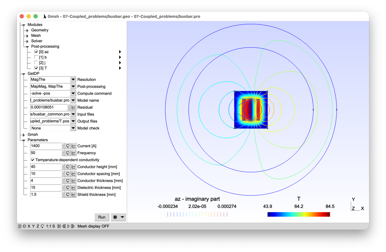
2.7.1 Features 
- Global currents and voltages in 2D a-v magneto-quasistatics
- Magneto-thermal resolution with multiphysics coupling
- Staggered resolution
See the comments in busbar.pro and busbar.geo for details.
2.7.2 Running the tutorial 
On the command line:
> gmsh busbar.geo -2
> getdp busbar.pro -solve MagThe -pos MapMag MapThe
Interactively with Gmsh: open busbar.pro with “File->Open”, then press “Run”.
2.7.3 Contents 
File busbar_common.pro 
mm = 1e-3;

DefineConstant[
  d = {10, Min 1, Max 100, Step 1,
    Name "Parameters/Conductor spacing [mm]"}
  e = {4, Min 1, Max 10, Step 1,
    Name "Parameters/Conductor thickness [mm]"}
  h = {40, Min 5, Max 100, Step 1,
    Name "Parameters/Conductor height [mm]"}
  g = {15, Min 1, Max 10, Step 1,
    Name "Parameters/Dielectric thickness [mm]"}
  t = {1.5, Min 1, Max 10, Step 1,
    Name "Parameters/Shield thickness [mm]"}
];

// Go back to meters:
d = d * mm;
e = e * mm;
h = h * mm;
g = g * mm;
t = t * mm;

// Internal and external radii of "infinite" region
rInt = 4 * (d + e + g + t);
rExt = 5.5 * (d + e + g + t);
File busbar.geo 
SetFactory("OpenCASCADE");

// Include the file with shared parameters, so that the same values are used
// here and in "busbar.pro":
Include "busbar_common.pro";

// Three rectangular conductors carrying balanced three-phase currents. The
// conductors are placed side by side, separated by a distance d, each with
// width e and height h:
For i In {1:3}
  Rectangle(i) = {-d - 1.5 * e + (i - 1) * (e + d), -h / 2, 0, e, h};
EndFor

// Insulation surrounding the three conductors, with a gap g on each side:
xx = -d - 1.5 * e - g;
yy = -h / 2 - g;
ww = 2 * d + 3 * e + 2 * g;
Rectangle(4) = {xx, yy, 0, ww, h + 2 * g};

// Metallic shield (thickness t) around the insulation:
Rectangle(5) = {xx - t, yy - t, 0, ww + 2 * t, h + 2 * g + 2 * t};

// Air region (disk) and infinite ring for the VolSphShell transformation (see
// tutorial 3); rInt and rExt are defined in "busbar_common.pro":
Disk(6) = {0, 0, 0, rInt};
Disk(7) = {0, 0, 0, rExt};

// Make all overlapping surfaces conformal (see tutorial 3):
Coherence;

// Mesh size constraints:
MeshSize { PointsOf{ Surface{6, 7}; } } = h / 5;
MeshSize { PointsOf{ Surface{4, 5}; } } = e / 3;
MeshSize { PointsOf{ Surface{1:3}; } } = e / 5;

// Physical groups:
Physical Surface("Conductor 1", 100) = {1};
Physical Surface("Conductor 2", 101) = {2};
Physical Surface("Conductor 3", 102) = {3};
Physical Surface("Insulator", 200) = {4};
Physical Surface("Shield", 201) = {5};
Physical Surface("Air", 202) = {6};
Physical Surface("Infinite shell", 203) = {7};

// Outermost boundary for the homogeneous Dirichlet boundary condition on the
// magnetic vector potential:
Physical Curve("Infinity", 300) = CombinedBoundary{ Surface{:}; };

// Boundary of all solid regions (conductors, insulator and shield) for the
// convection (Robin) boundary condition in the thermal problem:
Physical Curve("Convection", 301) = CombinedBoundary{ Surface{1:5}; };
File busbar.pro 
// This tutorial models the coupled magneto-thermal behavior of a three-phase
// busbar system, consisting of three conductors carrying balanced AC currents
// inside an insulating enclosure surrounded by a grounded metallic shield.
//
// The magnetic part solves a magneto-quasistatic problem (as in tutorial 4) in
// the frequency domain, using an "a-v" formulation that combines the magnetic
// vector potential "a" with an electric scalar potential "v". The electric
// scalar potential is introduced to handle conductors with imposed currents or
// voltages -- this extends the approach from tutorial 4 (which only had an
// imposed source current density) and from tutorial 6 (which introduced global
// quantities in an electrostatic context).
//
// More precisely, since "div b = 0", we start by introducing the vector
// potential "a" such that "b = curl a". Faraday's equation leads to "curl e =
// -\partial_t b = -\partial_t curl a", i.e. "curl (e + \partial_t a) = 0". We
// can thus derive "e + \partial_t a" from a scalar electric potential "v" such
// that "e + \partial_t a = -grad v".
//
// Whereas in tutorial 4 we fixed the gradient to zero (leading to the modified
// vector potential "a-formulation"), here we keep it in the conductors so that,
// in each conducting region, the electric field is expressed as
//
//   e = -\partial_t a - grad v,
//
// where "grad v" is assumed to be a constant (region-wise) vector along the
// z-axis in this 2D model. The current density in each conductor is then
//
//   j = sigma e = sigma (-\partial_t a - grad v).
//
// Integrating "j" over the cross-section of a conductor yields the total
// current, which can be imposed as a constraint. Similarly, the voltage drop
// per unit length along "z" can be imposed or computed. This is the "a-v"
// formulation, where "v" is discretized with a single global degree of freedom
// per conducting region.
//
// The thermal part solves the steady-state heat equation (as in tutorial 2),
// with time-averaged Joule losses from the magnetic solution as a volumetric
// heat source. Convection boundary conditions evacuate the heat on the outer
// surfaces of the solid regions.
//
// The coupling arises because the electrical conductivity "sigma" depends on
// temperature, and the Joule losses depend on the current distribution (which
// depends on "sigma"). A fixed-point (Picard) iteration (see tutorial 3)
// alternates between the magnetic and thermal solves until convergence.

Group {
  // Physical regions:
  Cond_1 = Region[ 100 ];
  Cond_2 = Region[ 101 ];
  Cond_3 = Region[ 102 ];
  Conds = Region[ {Cond_1, Cond_2, Cond_3} ];
  Insulator = Region[ 200 ];
  Shield = Region[ 201 ];
  Air = Region[ 202 ];
  AirInf = Region[ 203 ];
  Surface_Inf = Region[ 300 ];
  Surface_Conv = Region[ 301 ];

  // Abstract magnetic regions:
  //  - "Vol_Mag": full domain for the magnetic problem
  //  - "Vol_C_Mag": conducting regions where eddy currents and/or imposed
  //    currents flow (both the three-phase conductors and the grounded shield)
  //  - "Vol_Inf_Mag": region with infinite shell geometric transformation (see
  //    tutorial 3)
  //  - "Sur_Neu_Mag": surface with non-homogeneous Neumann conditions (empty
  //    here)
  Vol_Mag = Region[ {Conds, Insulator, Shield, Air, AirInf} ];
  Vol_C_Mag = Region[ {Conds, Shield} ];
  Vol_Inf_Mag = Region[ AirInf ];
  Sur_Neu_Mag = Region[ {} ];

  // Abstract thermal regions:
  //  - "Vol_The": domain for the thermal problem (solid regions only)
  //  - "Sur_Neu_The": surface with non-homogeneous Neumann conditions (empty)
  //  - "Sur_Rob_The": surface with Robin (convection) boundary condition
  Vol_The = Region[ {Conds, Insulator, Shield} ];
  Sur_Neu_The = Region[ {} ];
  Sur_Rob_The = Region[ {Surface_Conv} ];
}

Function {
  DefineConstant[
    Current = {1400, Min 1, Max 10000, Step 1,
      Name "Parameters/0Current [A]"}
    f = {50, Min 1, Max 1000, Step 1,
      Name "Parameters/1Frequency"}
    NonLinear = {1, Choices{0, 1},
      Name "Parameters/3Temperature-dependent conductivity" }
  ];

  // Magnetic parameters:
  mu0 = 4 * Pi * 1e-7;
  nu[] = 1. / mu0;

  If(NonLinear)
    // Temperature-dependent electrical conductivity of the copper conductors:
    // the argument "$1" will receive the local temperature value at runtime,
    // which is passed through "sigma[{T}]" in the Formulation (see below). This
    // is the mechanism through which the thermal solution influences the
    // magnetic problem:
    sigma[ Conds ] = 5.8e7 / (1 + 0.00393 * ($1 - 20));
  Else
    // Temperature independent electrical conductivity, for comparison purposes:
    sigma[ Conds ] = 5.8e7;
  EndIf

  // The electrical conductivity of the shield is assumed to be temperature
  // independent:
  sigma[ Shield ] = 3.5e7;

  // "CoefGeo[]" encodes the out-of-plane extent implicit in a 2D model:
  //   - for a planar 2D model, "CoefGeo == L", the out-of-plane length along
  //     the z-axis;
  //   - for an axisymmetric model, "CoefGeo == 2 * Pi" (the full revolution).
  // Its role in the a-v formulation, and why its sign matters, will be
  // explained below. In the present 2D model we set "L = +1 m", so
  // per-unit-length quantities are recovered directly:
  CoefGeo[] = 1;

  // Thermal parameters -- "k" is the thermal conductivity, "h" the convection
  // heat-transfer coefficient and "T0" the ambient temperature:
  k[ Conds ] = 385;
  k[ Shield ] = 205;
  k[ Insulator ] = 1;
  h[] = 60;
  T0[] = 20;

  // Tolerances and maximum iterations for the magneto-thermal fixed-point loop,
  // in the nonlinear case:
  NLTolAbs = 1e-12;
  NLTolRel = 1e-6;
  NLIterMax = 20;
}

Constraint {
  // Homogeneous Dirichlet condition on the magnetic vector potential at infinity
  // (as in tutorials 3 and 4):
  { Name a_Mag_2D;
    Case {
      { Region Surface_Inf; Value 0; }
    }
  }

  // Imposed total current in each conductor. The three-phase balanced currents
  // are specified with 120 degree phase shifts using the built-in function
  // "F_Cos_wt_p[]{omega, phi}", which is interpreted as "Complex[Cos[phi],
  // Sin[phi]]" in the frequency domain (and as "Cos[omega * $Time + phi]" in
  // the time domain -- see tutorial 4 for a similar mechanism with
  // "F_Sin_wt_p[]"):
  { Name Current_Mag_2D;
    Case {
      { Region Cond_1; Value Current;
        TimeFunction F_Cos_wt_p[]{2 * Pi * f, 0}; }
      { Region Cond_2; Value Current;
        TimeFunction F_Cos_wt_p[]{2 * Pi * f, -2 * Pi / 3}; }
      { Region Cond_3; Value Current;
        TimeFunction F_Cos_wt_p[]{2 * Pi * f, 2 * Pi / 3}; }
    }
  }

  // The shield is grounded, i.e. zero voltage drop along the z-axis. This
  // allows induced (eddy) currents to flow freely in the shield, driven by the
  // time-varying magnetic flux:
  { Name Voltage_Mag_2D;
    Case {
      { Region Shield; Value 0; }
    }
  }

  // Initial temperature for the thermal problem:
  { Name T_The; Type Init;
    Case {
      { Region Vol_The; Value T0[]; }
    }
  }
}

// Import the values of "rInt" and "rExt" for the infinite shell Jacobian:
Include "busbar_common.pro";

Jacobian {
  { Name Vol;
    Case {
      // Use the infinite shell Jacobian on the annular region:
      { Region Vol_Inf_Mag; Jacobian VolSphShell{rInt, rExt}; }
      { Region All; Jacobian Vol; }
    }
  }
  { Name Sur;
    Case {
      { Region All; Jacobian Sur; }
    }
  }
}

Integration {
  { Name Int;
    Case {
      { Type Gauss;
        Case {
          { GeoElement Line; NumberOfPoints 4; }
          { GeoElement Triangle; NumberOfPoints 4; }
        }
      }
    }
  }
}

Group {
  Dom_Hcurl_a_Mag_2D = Region[ {Vol_Mag, Sur_Neu_Mag} ];
  Dom_H1_T_The = Region[ {Vol_The, Sur_Neu_The, Sur_Rob_The} ];
}

FunctionSpace {
  // Magnetic vector potential, discretized as in tutorials 3 and 4 with
  // perpendicular edge basis functions "BF_PerpendicularEdge" associated with
  // the nodes of the mesh:
  { Name Hcurl_a_Mag_2D; Type Form1P;
    BasisFunction {
      { Name se; NameOfCoef ae; Function BF_PerpendicularEdge;
        Support Dom_Hcurl_a_Mag_2D; Entity NodesOf[All]; }
    }
    Constraint {
      { NameOfCoef ae; EntityType NodesOf; NameOfConstraint a_Mag_2D; }
    }
  }

  // The gradient of the electric scalar potential, "grad v", is discretized
  // with one global degree of freedom per conducting region using the
  // "BF_RegionZ" basis function. "BF_RegionZ" is the unit vector along the
  // z-axis -- constant and equal to "(0, 0, 1)" -- on each region in
  // "Vol_C_Mag", and zero everywhere else. It is the vector counterpart of the
  // scalar "BF_GroupOfNodes" basis function introduced in tutorial 6 for global
  // quantities.
  //
  // The finite element expansion of "grad v" thus reads
  //
  //   grad v = Sum_{r in Vol_C_Mag} ur_r sr_r(x, y)
  //
  // where "ur_r" is the (constant, complex-valued) z-component of the gradient
  // of the electric potential in region r, and "sr_r(x, y)" is the unit vector
  // along z, equal to 1 in region r and 0 elsewhere.
  //
  // As with the electrostatic global quantities in tutorial 6, the voltage
  // ("AliasOf") and the current ("AssociatedWith") are energy duals. The rule
  // of thumb when choosing which gets which type: the quantity that plays the
  // role of the primary degree of freedom -- the one the variational
  // formulation uses as test function -- is the "AliasOf"; its energy-dual (the
  // quantity that appears in the bilinear form paired with the test function)
  // is the "AssociatedWith". Accordingly, the GlobalTerm below pairs "Dof{I}"
  // (AssociatedWith) with "{U}" (AliasOf), exactly the way "GlobalTerm
  // [-Dof{Q}, {V}]" pairs charge with voltage in tutorial 6.
  { Name Hcurl_u_Mag_2D; Type Form1P;
    BasisFunction {
      // constant vector over the region, with only nonzero z-component
      { Name sr; NameOfCoef ur; Function BF_RegionZ;
        Support Vol_C_Mag; Entity Vol_C_Mag; }
    }
    GlobalQuantity {
      { Name Voltage; Type AliasOf; NameOfCoef ur; }
      { Name Current; Type AssociatedWith; NameOfCoef ur; }
    }
    Constraint {
      { NameOfCoef Voltage; EntityType Region; NameOfConstraint Voltage_Mag_2D; }
      { NameOfCoef Current; EntityType Region; NameOfConstraint Current_Mag_2D; }
    }
  }

  // Temperature, discretized with standard nodal (Lagrange) basis functions (as
  // in tutorial 2):
  { Name H1_T_The; Type Form0;
    BasisFunction {
      { Name sn; NameOfCoef Tn; Function BF_Node; Support Dom_H1_T_The;
        Entity NodesOf[All]; }
    }
    Constraint {
      { NameOfCoef Tn; EntityType NodesOf; NameOfConstraint T_The; }
    }
  }

}

Formulation {
  // Magneto-quasistatic a-v formulation.
  //
  // Using the constitutive law "h = nu b" together with "b = curl a" in
  // Ampere's equation, and plugging Ohm's law "j = sigma e" with "e =
  // -\partial_t a - grad v", we obtain
  //
  //   curl(nu curl a) = j = sigma e = -sigma \partial_t a - sigma grad v.
  //
  // In each conducting region, "grad v" is assumed to be constant, and zero
  // everywhere else. The weak a-v formulation then reads: find "a" and "v" such
  // that
  //
  //   (nu curl a, curl a')_Vol_Mag + (sigma \partial_t a, a')_Vol_C_Mag
  //     + (sigma grad v, a')_Vol_C_Mag = 0
  //
  //   - (sigma \partial_t a, ur')_Vol_C_Mag - (sigma grad v, ur')_Vol_C_Mag
  //     = I(ur')
  //
  // hold for all test functions "a'" and "ur'", with "I(ur') = I_r", the
  // current in conductor "r", for each "r" in "Vol_C_Mag". For each test
  // function "sr_r" (the global basis function for conductor "r"), the second
  // equation yields the circuit relation linking the voltage drop and the
  // current in region "r". In the first equation, as in tutorial 4, the
  // boundary term resulting from integration by parts vanishes since "a" is set
  // to 0 on the boundary of "Vol_Mag".
  //
  // In order to account for the out-of-plane length "L" of the model, we define
  // "grad v = ur / CoefGeo[]". Here "{ur}" is the discrete DoF attached to
  // "BF_RegionZ" (a constant z-vector per conducting region); dividing by
  // "CoefGeo[]" converts the region-wise voltage drop to the physical gradient
  // that appears in the PDE. "CoefGeo[]" plays two roles:
  //  - Everywhere "grad v" enters an integrand, it is written as "{ur} /
  //    CoefGeo[]", with "CoefGeo == L" in planar 2D and "CoefGeo == 2 * Pi" in
  //    axisymmetric. This is a modelling convention, not a Jacobian correction:
  //    the "Vol" (resp. "VolAxi") Jacobian already rescales each surface
  //    integrand to its 3D counterpart. So "CoefGeo" divides "{ur}" in
  //    "Integral" terms only where "grad v" appears explicitly.
  //  - The sign of "CoefGeo[]" lets the user flip the orientation of the
  //    current in a region (e.g. for a return conductor). This sign enters the
  //    circuit relation via the "GlobalTerm" with "Sign[CoefGeo[]]" below. In
  //    the present 2D model, "CoefGeo[] = 1", so the sign has no numerical
  //    effect -- it is kept so that the same formulation can be reused in
  //    models with oppositely-oriented conductors.
  { Name Magnetoquasistatics_av_2D; Type FemEquation;
    Quantity {
      { Name a; Type Local; NameOfSpace Hcurl_a_Mag_2D; }
      { Name ur; Type Local; NameOfSpace Hcurl_u_Mag_2D; }
      { Name I; Type Global; NameOfSpace Hcurl_u_Mag_2D [Current]; }
      { Name U; Type Global; NameOfSpace Hcurl_u_Mag_2D [Voltage]; }

      // Declaring "T" in this formulation gives access to the temperature field
      // from the thermal FunctionSpace, which is needed to evaluate the
      // temperature-dependent conductivity sigma:
      { Name T; Type Local; NameOfSpace H1_T_The; }
    }
    Equation {
      Integral { [ nu[] * Dof{d a} , {d a} ];
        In Vol_Mag; Jacobian Vol; Integration Int; }
      // The coefficients in the magneto-quasistatic formulation will be
      // complex-valued, while those in the thermal formulation will be
      // real-valued. The "<T>[ ... ]" syntax instructs GetDP to evaluate the
      // expression inside in real arithmetic (in the FunctionSpace of "T"),
      // even though the formulation is complex-valued:
      Integral { DtDof [ sigma[<T>[{T}]] * Dof{a} , {a} ];
        In Vol_C_Mag; Jacobian Vol; Integration Int; }
      Integral { [ sigma[<T>[{T}]] * Dof{ur} / CoefGeo[] , {a} ];
        In Vol_C_Mag; Jacobian Vol; Integration Int; }

      Integral { DtDof [ sigma[<T>[{T}]] * Dof{a} , {ur} ];
        In Vol_C_Mag; Jacobian Vol; Integration Int; }
      Integral { [ sigma[<T>[{T}]] * Dof{ur} / CoefGeo[] , {ur} ];
        In Vol_C_Mag; Jacobian Vol; Integration Int; }
      // "Sign[CoefGeo[]]" accounts for a possible sign reversal of the current
      // direction (when "CoefGeo[] < 0"):
      GlobalTerm { [ Dof{I} * Sign[CoefGeo[]] , {U} ]; In Vol_C_Mag; }
    }
  }

  // Thermal formulation.
  //
  // We proceed as in tutorial 2, but in steady state and with a volume heat
  // source "Q". The steady-state thermal conduction problem is governed by
  //
  //    - div(k grad T) = Q,
  //
  // which, with the same convection boundary condition as in tutorial 2, leads
  // to the following weak form: find "T" such that
  //
  //   (k grad T, grad T')_Vol_The + (h (T - T0), T')_Sur_Rob_The
  //     = (Q, T')_Vol_C_Mag
  //
  // holds for all test functions "T'". In our magneto-thermal setting, "Q" is
  // the time-averaged Joule loss density over a period "[0, Tp]":
  //
  //   Q = 1/Tp \int_0^Tp sigma |e(t)|^2 dt = sigma/2 |E|^2
  //
  // with "E" the complex phasor of the electric field (the factor 1/2 comes
  // from time-averaging the squared sinusoid).

  { Name Thermal_T; Type FemEquation;
    Quantity {
      { Name T; Type Local; NameOfSpace H1_T_The; }

      // Declaring "{a}" and "{ur}" here gives access to the magnetic solution
      // (computed in the frequency domain) in order to evaluate Joule losses:
      { Name a; Type Local; NameOfSpace Hcurl_a_Mag_2D; }
      { Name ur; Type Local; NameOfSpace Hcurl_u_Mag_2D; }
    }
    Equation {
      Integral { [ k[] * Dof{d T} , {d T} ];
        In Vol_The; Jacobian Vol; Integration Int; }

      Integral { [ h[] * Dof{T} , {T} ];
        In Sur_Rob_The; Jacobian Sur; Integration Int; }
      Integral { [ -h[] * T0[] , {T} ];
        In Sur_Rob_The; Jacobian Sur; Integration Int; }

      // The "<a>[ ... ]" syntax instructs GetDP to evaluate the expression
      // inside in complex arithmetic, even though the thermal formulation is
      // real-valued. Without it, only the real part of "{a}" and "{ur}" would
      // be used, which would give incorrect results. Note that, at the point
      // the thermal system is assembled, "{a}" and "{ur}" refer to the magnetic
      // solution that has already been computed (there is no "Dof" prefix),
      // i.e. they refer to known phasor fields. The expression "SquNorm[...]"
      // computes the squared modulus "|...|^2 = Re[...]^2 + Im[...]^2":
      Integral { [ -0.5 * sigma[{T}] * <a>[SquNorm[Dt[{a}] + {ur} / CoefGeo[]]],
          {T} ]; In Vol_C_Mag; Jacobian Vol; Integration Int; }
    }
  }
}

Resolution {
  // The coupled magneto-thermal resolution alternates between the magnetic and
  // thermal solves. The coupling is through:
  //  1) "sigma[{T}]": the conductivity in the magnetic problem depends on "T";
  //  2) Joule losses: the heat source "Q" in the thermal problem depends on the
  //     magnetic solution ("a", "ur").
  //
  // This is a fixed-point (Picard) iteration scheme: at each iteration, the
  // magnetic system is solved with the current temperature distribution, then
  // the thermal system is solved with the resulting Joule losses. The process
  // repeats until the magnetic residual converges (indicating self-consistency
  // of the two coupled problems).
  //
  // A monolithic coupling could also be implemented, where a single coupled
  // system is solved.
  //
  // If the NonLinear flag is not set, we disregard the temperature dependency
  // of copper conductivity and the coupled problem can be solved without
  // iterating.
  { Name MagThe;
    System {
      // The magnetic system is complex-valued and solved at a single frequency
      // (as in the frequency-domain case of tutorial 4):
      { Name Sys_Mag; NameOfFormulation Magnetoquasistatics_av_2D;
        Type Complex; Frequency f; }
      // The thermal system is real-valued:
      { Name Sys_The; NameOfFormulation Thermal_T; }
    }
    Operation {
      // Initialize the temperature to the initial condition "T0[]":
      InitSolution[Sys_The];

      // First solve: magnetic with the initial temperature, then thermal:
      Generate[Sys_Mag]; Solve[Sys_Mag];
      Generate[Sys_The]; Solve[Sys_The];

      If(NonLinear)
        // Re-generate the magnetic system with the updated temperature (which
        // changes sigma), and compute the initial residual:
        Generate[Sys_Mag];
        GetResidual[Sys_Mag, $res0];

        // Initialize runtime variables to track the residual and the iteration
        // count, then print out the absolute and relative residual:
        Evaluate[ $res = $res0, $iter = 0 ];
        Print[{$iter, $res, $res / $res0},
          Format "Residual %03g: abs %14.12e rel %14.12e"];

        // Iterate until convergence (same loop structure as in tutorial 3):
        While[$res > NLTolAbs && $res / $res0 > NLTolRel &&
          $res / $res0 <= 1 && $iter < NLIterMax]{
          Solve[Sys_Mag];
          Generate[Sys_The]; Solve[Sys_The];
          Generate[Sys_Mag]; GetResidual[Sys_Mag, $res];
          Evaluate[ $iter = $iter + 1 ];
          Print[{$iter, $res, $res / $res0},
            Format "Residual %03g: abs %14.12e rel %14.12e"];
        }
      EndIf

      SaveSolution[Sys_Mag];
      SaveSolution[Sys_The];
    }
  }
}

PostProcessing {
  // Post-processing for the magnetic formulation. Since the magnetic solution
  // is complex-valued, all quantities defined here are complex phasors:
  { Name Mag; NameOfFormulation Magnetoquasistatics_av_2D;
    Quantity {
      { Name a;
        Value {
          Term { [ {a} ]; In Vol_Mag; Jacobian Vol; }
        }
      }
      { Name az;
        Value {
          Term { [ CompZ[{a}] ]; In Vol_Mag; Jacobian Vol; }
        }
      }
      { Name b;
        Value {
          Term { [ {d a} ]; In Vol_Mag; Jacobian Vol; }
        }
      }
      { Name j;
        Value {
          Term { [ -sigma[<T>[{T}]] * (Dt[{a}] + {ur} / CoefGeo[]) ];
            In Vol_C_Mag; Jacobian Vol; }
        }
      }
      { Name JouleLosses;
        Value {
          Integral { [ 0.5 * sigma[<T>[{T}]] * SquNorm[Dt[{a}] + {ur} /
                CoefGeo[]] ]; In Vol_C_Mag; Jacobian Vol; Integration Int; }
        }
      }
      { Name U;
        Value {
          Term { [ {U} ]; In Vol_C_Mag; }
        }
      }
      { Name I;
        Value {
          Term { [ {I} ]; In Vol_C_Mag; }
        }
      }
    }
  }

  // Post-processing for the thermal formulation:
  { Name The; NameOfFormulation Thermal_T;
    Quantity {
      { Name T;
        Value {
          Term { [ {T} ]; In Vol_The; Jacobian Vol; }
        }
      }
    }
  }
}

PostOperation {
  { Name MapMag; NameOfPostProcessing Mag;
    Operation {
      Print[ az, OnElementsOf Vol_Mag, File "az.pos" ];
      Print[ b, OnElementsOf Vol_Mag, File "b.pos" ];
      Print[ j, OnElementsOf Vol_C_Mag, File "j.pos" ];
      // "RegionTable" outputs one row per region (instead of one row per
      // element), which is appropriate for global quantities:
      Print[ U, OnRegion Vol_C_Mag, File "U.txt", Format RegionTable ];
      Print[ I, OnRegion Vol_C_Mag, File "I.txt", Format RegionTable ];
    }
  }
  { Name MapThe; NameOfPostProcessing The;
    Operation {
      Print[ T, OnElementsOf Vol_The, File "T.pos" ];
    }
  }
}

// Setting a variable with the reserved name "GetDP/2PostOperationChoices"
// allows to control which PostOperations are performed by default by Gmsh
// when the model is run interactively. Here we request both "MapMag" and
// "MapThe", instead of just "MapMag" (the default):
DefineConstant[
  PostOp = {"MapMag, MapThe", Name "GetDP/2PostOperationChoices"}
];
2.8 Tutorial 8: Circuit coupling in 2D and 3D 
Two conductors modeled with finite elements are connected in parallel and driven by a voltage source through a series resistance and inductance. The lumped circuit elements and the finite element conductors are coupled through a network constraint that enforces Kirchhoff’s laws via a global equation. In 3D, the vector potential is discretized with Whitney edge elements and a tree-cotree gauge ensures uniqueness. Both frequency-domain and time-domain analyses are supported.
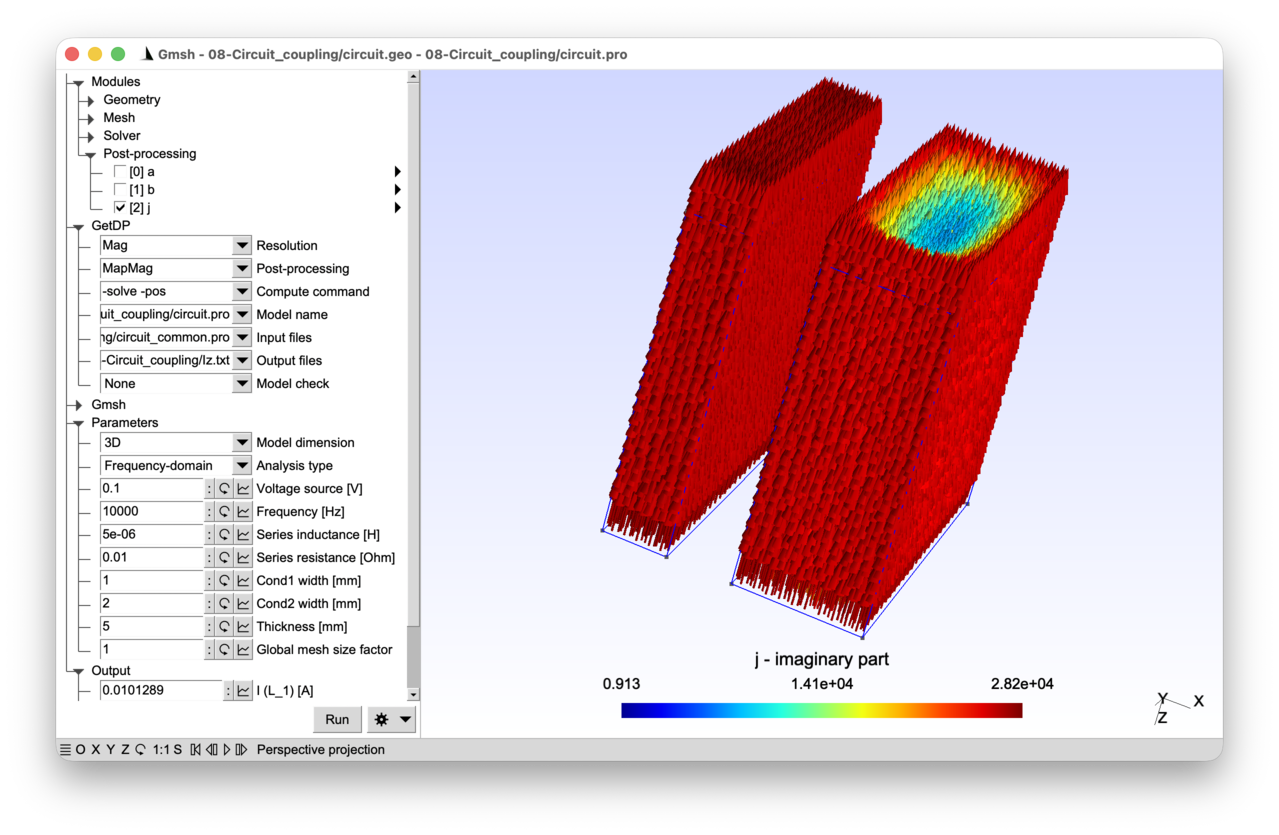
2.8.1 Features 
- Circuit coupling in 2D and 3D a-v magneto-quasistatics
- Lumped resistors, inductors and voltage sources
- Discretization of the 3D vector potential with tree-cotree gauging
- Gradient basis functions for the 3D electric scalar potential
See the comments in circuit.pro and circuit.geo for details.
2.8.2 Running the tutorial 
On the command line (2D analysis):
> gmsh circuit.geo -2
> getdp circuit.pro -solve Mag -pos MapMag
On the command line (3D analysis):
> gmsh circuit.geo -3 -setnumber dim 3
> getdp circuit.pro -solve Mag -pos MapMag -setnumber dim 3
Interactively with Gmsh: open circuit.pro with “File->Open”, then press “Run”.
2.8.3 Contents 
File circuit_common.pro 
DefineConstant[
  dim = {2, Choices{2="2D", 3="3D"},
    Name "Parameters/0Model dimension"}
  thick = {5, Min 0.1, Max 10, Step 0.1,
    Name "Parameters/Thickness [mm]"}
];

// back to meters:
mm = 1e-3;
thick = thick * mm;
File circuit.geo 
// Gmsh script describing the geometry of two rectangular conductors. In 2D the
// model consists of two rectangles (cross-sections of the conductors). In 3D
// the rectangles are extruded along z to form volumes, and the bottom and top
// surfaces of each conductor are identified as separate physical groups: these
// will serve as electrodes in the 3D circuit coupling.

SetFactory("OpenCASCADE");

Include "circuit_common.pro";

DefineConstant[
  w1 = {1, Min 0.1, Max 10, Step 0.1,
    Name "Parameters/Cond1 width [mm]"}
  w2 = {2, Min 0.1, Max 10, Step 0.1,
    Name "Parameters/Cond2 width [mm]"}
  s = {1, Min 0.1, Max 10, Step 0.1,
    Name "Parameters/}Global mesh size factor"}
];

w1 = w1 * mm;
w2 = w2 * mm;
h = 5 * mm;

Rectangle(1) = {0, 0, 0, w1, h};
Rectangle(2) = {w1 + 1 * mm, 0, 0, w2, h};

If(dim == 3)
  // Extrude both rectangles along z. The "Extrude" command returns a list: the
  // first element (index 0) is the top surface, and the second (index 1) is the
  // newly created volume:
  left() = Extrude{0, 0, thick}{ Surface{1}; };
  cond1 = left(1);
  right() = Extrude{0, 0, thick}{ Surface{2}; };
  cond2 = right(1);
Else
  cond1 = 1;
  cond2 = 2;
EndIf

MeshSize{:} = 0.2 * mm * s;

bnd() = CombinedBoundary{ GeoEntity{dim}{:}; };

Physical GeoEntity{dim}("Conductor 1", 100) = cond1;
Physical GeoEntity{dim}("Conductor 2", 101) = cond2;
Physical GeoEntity{dim - 1}("Boundary", 200) = bnd();

If(dim == 3)
  // The bottom and top surfaces of each conductor are needed as electrode
  // surfaces for the 3D a-v formulation with circuit coupling. Surface tag "1"
  // is the original rectangle (bottom of cond1), and "left(0)" is the top
  // surface created by the extrusion. Similarly for cond2:
  Physical Surface("Bottom left", 300) = 1;
  Physical Surface("Top left", 301) = left(0);
  Physical Surface("Bottom right", 302) = 2;
  Physical Surface("Top right", 303) = right(0);
EndIf
File circuit.pro 
// This tutorial shows how to couple a finite element model with a lumped
// element circuit. We consider two conductors (modelled with finite elements)
// connected in parallel and driven by a voltage source through a series
// resistance and inductance (modelled as lumped circuit elements). The circuit
// topology is described as follows (with circled numbers representing the
// circuit nodes):
//
//    (2)     +-----+   (3)   +-----+       (4)
//     +------+ R_1 +----+----+ L_1 +--------+------------+
//     |      +-----+         +-----+        |            |
//     |                                +----+----+  +----+----+
//  +--+--+                             |         |  |         |
//  | V_1 |                             | Cond_1  |  | Cond_2  |
//  +--+--+                             |         |  |         |
//     |                                +----+----+  +----+----+
//     |                                     |            |
//     +-------------------------------------+------------+
//    (1)
//
// The two conductors "Cond_1" and "Cond_2" are discretized with finite
// elements, while "V_1" (voltage source), "R_1" (resistance) and "L_1"
// (inductance) are lumped circuit elements.
//
// Both the 2D and the 3D cases are treated using an "a-v" magneto-quasistatic
// formulation in the conductors, which takes into account skin effect.
// Proximity effects are not modelled, as the magnetic problem is only solved in
// the conductors: there is no surrounding air region, so the two conductors are
// magnetically uncoupled.
//
// In 2D, the magnetic vector potential "a" is a perpendicular 1-form
// ("Form1P"), as in tutorials 4 and 7, and the electric scalar potential "v" is
// discretized with a single global degree of freedom per conducting region, as
// in tutorial 7. In 3D, "a" is a 1-form ("Form1") discretized with Whitney edge
// elements, as in tutorial 5. The electric scalar potential "v" is now a full
// scalar field inside each conductor, whose gradient is discretized with
// "BF_GradNode" (the gradient of the standard Lagrange basis functions) and
// "BF_GradGroupOfNodes" (the gradient of the global basis functions introduced
// in tutorial 6). An explicit gauge condition (tree-cotree gauging) is needed
// to remove the gradient fields from "a", which would otherwise be redundant
// with "grad v" (see below).
//
// Both frequency-domain and time-domain analyses are supported (as in tutorial
// 4).

Include "circuit_common.pro";

Group {
  // Physical regions (in the mesh):
  Cond_1 = Region[ 100 ];
  Cond_2 = Region[ 101 ];
  Bnd = Region[ 200 ];
  If(dim == 3)
    BotCond_1 = Region[ 300 ];
    TopCond_1 = Region[ 301 ];
    BotCond_2 = Region[ 302 ];
    TopCond_2 = Region[ 303 ];
  EndIf

  // Circuit regions. These are fictitious regions used to represent lumped
  // circuit elements. Their tags must not conflict with any physical group tag
  // in the mesh, so that GetDP can distinguish them from mesh-based regions:
  V_1 = Region[ 1000 ];
  R_1 = Region[ 1001 ];
  L_1 = Region[ 1002 ];

  // Abstract magnetic regions:
  //  - "Vol_Mag": full domain for the magnetic problem
  //  - "Vol_C_Mag": conducting regions
  //  - "Sur_Electrodes_Mag": electrode surfaces with voltages and currents in
  //    3D
  Vol_Mag = Region[ {Cond_1, Cond_2} ];
  Vol_C_Mag = Region[ {Cond_1, Cond_2} ];
  If(dim == 3)
    Sur_Electrodes_Mag = Region[ {BotCond_1, TopCond_1, BotCond_2, TopCond_2} ];
  EndIf

  // Abstract circuit regions. These groups allow a generic treatment of the
  // lumped element constitutive relations in the Formulation (see the
  // GlobalTerms below):
  //  - "Resistance_Cir": resistors (U = R I)
  //  - "Inductance_Cir": inductors (U = L dI/dt)
  //  - "Capacitance_Cir": capacitors (I = C dU/dt)
  //  - "Dom_Cir": all lumped circuit elements
  Resistance_Cir = Region[ {R_1} ];
  Inductance_Cir = Region[ {L_1} ];
  Capacitance_Cir = Region[ {} ]; // empty, but kept for completeness
  Dom_Cir = Region[ {V_1, R_1, L_1} ];
}

Function {
  DefineConstant[
    AnalysisType = {1, Choices{0="Time-domain", 1="Frequency-domain"},
      Name "Parameters/1Analysis type"}
    Voltage = {0.1, Min 1e-3, Max 10, Step 1,
      Name "Parameters/2Voltage source [V]"}
    // In the frequency domain we consider an AC voltage source with frequency
    // "f":
    f = {1000, Min 1, Max 10000, Step 10, Visible AnalysisType == 1,
      Name "Parameters/3Frequency [Hz]"}
    // In the time domain we consider a step voltage with given rise time "tr",
    // and run the simulation for "10 * tr":
    tr = {1e-3, Min 1e-5, Max 1, Step 1e-3, Visible AnalysisType == 0,
      Name "Parameters/3Rise time"}
    Rval = {10e-3, Min 0, Max 100, Step 0.1,
      Name "Parameters/4Series resistance [Ohm]"}
    Lval = {5e-6, Min 0, Max 100e-6, Step 1e-6,
      Name "Parameters/4Series inductance [H]"}
  ];

  If(AnalysisType == 1)
    tfct[] = F_Cos_wt_p[]{2 * Pi * f, 0};
  Else
    tmax = 10 * tr;
    dt = tr / 10;
    // A simple ramp function for the step voltage:
    tfct[] = ($Time < tr) ? $Time / tr : 1;
  EndIf

  // Magnetic parameters:
  mu0 = 4 * Pi * 1e-7;
  nu[] = 1. / mu0;
  sigma[ Cond_1 ] = 5.8e7;
  sigma[ Cond_2 ] = 5.8e7;

  If(dim == 2)
    // In 2D, "CoefGeo[]" represents the out-of-plane thickness (as in tutorial
    // 7):
    CoefGeo[] = thick;
  Else
    // In 3D the thickness is part of the geometrical model and the mesh, so
    // "CoefGeo[] = 1":
    CoefGeo[] = 1;
  EndIf

  // Circuit parameters: the "Resistance[]", "Inductance[]" and "Capacitance[]"
  // functions are piecewise constants defined on the circuit regions, used in
  // the lumped element GlobalTerms of the Formulation:
  Resistance[ R_1 ] = Rval;
  Inductance[ L_1 ] = Lval;
  Capacitance[ ] = 0; // unused
}

Constraint {
  // Homogeneous Dirichlet condition on the magnetic vector potential on the
  // outer boundaries:
  { Name a_Mag;
    Case {
      { Region Bnd; Value 0.; }
    }
  }

  // Tree-cotree gauge condition for the 3D vector potential (see the
  // FunctionSpace definition below for details):
  { Name a_Gauge_Mag;
    Case {
      { Region Vol_C_Mag ; SubRegion Bnd; Value 0.; }
    }
  }

  // No imposed current constraint on the FE conductors (the current will be
  // determined by the circuit):
  { Name Current_Mag;
    Case {
    }
  }

  { Name Voltage_Mag;
    Case {
      If(dim == 3)
        // In 3D, set the absolute voltage on the bottom electrode of "Cond_1"
        // to 0 as a reference:
        { Region BotCond_1; Value 0; }
      EndIf
    }
  }

  // Initial condition on the circuit inductor current (for the time-domain
  // analysis):
  { Name Current_Cir ;
    Case {
      { Region L_1; Type Init; Value 0.; }
    }
  }

  // Imposed voltage on the voltage source:
  { Name Voltage_Cir ;
    Case {
      { Region V_1; Value Voltage; TimeFunction tfct[]; }
    }
  }

  // The circuit topology is described as a constraint of type "Network". Each
  // entry specifies a circuit element (a "Region") and the two circuit nodes
  // ("Branch") it connects, defining a directed branch from the first node to
  // the second. The circuit node numbers (1, 2, 3, 4, ...) are arbitrary labels
  // that refer to the ASCII art diagram at the top of this file.
  //
  // The sign convention is the same for all elements (sources and loads alike):
  // for a branch "Branch {a, b}", the current "I" is positive from node "a" to
  // node "b", and the voltage "U" is the potential rise from "a" to "b", i.e.
  // "U = V(b) - V(a)". This uniform "source" (or "generator") convention
  // differs from the "passive sign convention" commonly used in circuit
  // textbooks, where the current through a load is defined as flowing into the
  // positive voltage terminal.
  //
  // The constitutive law of each element determines the relation between "U"
  // and "I". With the source convention:
  //   - Resistor: U + R I = 0 (voltage drops in the direction of current)
  //   - Inductor: U + L dI/dt = 0
  //   - Capacitor: I + C dU/dt = 0
  //   - Voltage source: U = Voltage * tfct[] (via the "Voltage_Cir" constraint)
  //
  // The power delivered by any element is "P = U I": sources have "P > 0" and
  // loads have "P < 0" (e.g. for a resistor, "P = U I = -R I^2 < 0").
  { Name ElectricalCircuit ; Type Network ;
    Case Circuit_1 {
      // Lumped elements:
      { Region V_1; Branch {1, 2}; }
      { Region R_1; Branch {2, 3}; }
      { Region L_1; Branch {3, 4}; }

      If(dim == 2)
        // In 2D, each conducting region has a single voltage drop and current
        // flowing through it (in the direction perpendicular to the plane). It
        // behaves as a two-terminal circuit element and can be directly
        // inserted between two circuit nodes. Here both conductors are
        // connected in parallel between nodes 4 and 1:
        { Region Cond_1; Branch {4, 1} ; }
        { Region Cond_2; Branch {4, 1} ; }
      Else
        // In 3D, each electrode surface carries a voltage (absolute potential)
        // and a current. To impose a voltage drop across a conductor (say
        // "Cond_1") in the circuit -- rather than an absolute voltage on each
        // electrode surface independently -- we use an "anti-serial"
        // connection.  The key idea is to connect the top and bottom electrodes
        // with opposite node orderings, so that their absolute voltages are
        // subtracted:
        //
        //   V_drop(Cond_1) = V(TopCond_1) - V(BotCond_1).
        //
        // This is achieved by connecting "TopCond_1" from node 4 to an
        // intermediate node 10, and "BotCond_1" from node 1 to the same node 10
        // (note the reversed direction). The voltage between nodes 4 and 1 then
        // corresponds to the voltage drop over "Cond_1", regardless of the
        // absolute voltage values. The current convention is also consistent:
        // the current flowing into "TopCond_1" equals the current flowing out
        // of "BotCond_1".
        //
        // Note: in this particular circuit, since "BotCond_1" is fixed at 0 V
        // through the "Voltage_Mag" constraint, the anti-serial connection for
        // the bottom face is not strictly necessary. However, it is included
        // here for generality. Beware that if the bottom face is removed from
        // the Network, the corresponding region "BotCond_1" has to be removed
        // from "Sur_Electrodes_Mag" as well!
        { Region TopCond_1; Branch {4, 10} ; }
        { Region BotCond_1; Branch {1, 10} ; }

        { Region TopCond_2; Branch {4, 11} ; }
        { Region BotCond_2; Branch {1, 11} ; }
      EndIf
    }
  }
}

Jacobian {
  { Name Vol;
    Case {
      { Region All; Jacobian Vol; }
    }
  }
  { Name Sur;
    Case {
      { Region All; Jacobian Sur; }
    }
  }
}

Integration {
  { Name Int;
    Case {
      { Type Gauss;
        Case {
          { GeoElement Line; NumberOfPoints 4; }
          { GeoElement Triangle; NumberOfPoints 4; }
          { GeoElement Tetrahedron; NumberOfPoints 4; }
        }
      }
    }
  }
}

FunctionSpace {
  If(dim == 2)
    // In 2D, the magnetic vector potential and the gradient of the electric
    // scalar potential are discretized as in tutorial 7:
    { Name Hcurl_a_Mag_2D; Type Form1P;
      BasisFunction {
        { Name se; NameOfCoef ae; Function BF_PerpendicularEdge;
          Support Vol_Mag; Entity NodesOf[All]; }
      }
      Constraint {
        { NameOfCoef ae; EntityType NodesOf; NameOfConstraint a_Mag; }
      }
    }
    { Name Hcurl_u_Mag_2D; Type Form1P;
      BasisFunction {
        { Name sr; NameOfCoef ur; Function BF_RegionZ;
          Support Vol_C_Mag; Entity Vol_C_Mag; }
      }
      GlobalQuantity {
        { Name Voltage; Type AliasOf; NameOfCoef ur; }
        { Name Current; Type AssociatedWith; NameOfCoef ur; }
      }
      Constraint {
        { NameOfCoef Voltage; EntityType Region; NameOfConstraint Voltage_Mag; }
        { NameOfCoef Current; EntityType Region; NameOfConstraint Current_Mag; }
      }
    }
  Else
    // In 3D, the magnetic vector potential is a true 1-form (Form1), as in
    // tutorial 5, discretized with Whitney edge basis functions "BF_Edge"
    // associated with the edges of the mesh:
    { Name Hcurl_a_Mag_3D; Type Form1;
      BasisFunction {
        { Name se; NameOfCoef ae; Function BF_Edge;
          Support Vol_Mag; Entity EdgesOf[All]; }
      }
      Constraint {
        { NameOfCoef ae; EntityType EdgesOf; NameOfConstraint a_Mag; }
        // Tree-cotree gauge condition for 3D. In the conducting regions, the
        // electric field "e = -\partial_t a - grad v" involves two unknowns,
        // "a" and "grad v", but only their sum matters physically. Since the
        // edge element space of "a" can represent arbitrary gradient fields,
        // any gradient could be moved freely between "a" and "grad v" without
        // changing "e": the system is thus singular without an additional
        // constraint.
        //
        // Tree-cotree gauging removes gradient fields from "a" by setting to
        // zero the degrees of freedom of "a" on the edges of a spanning tree of
        // the mesh graph in "Vol_C_Mag". The "EdgesOfTreeIn" entity type
        // selects such a tree, rooted on the boundary "Bnd" (specified by
        // "EntitySubType StartingOn") where "a" is already constrained to
        // zero. This action eliminates the irrotational (gradient) components
        // of "a", leaving only the solenoidal part; "ur" alone will carry the
        // gradient part of the electric field.
        //
        // See tutorial 10 for more details about gauging.
        { NameOfCoef ae; EntityType EdgesOfTreeIn; EntitySubType StartingOn;
          NameOfConstraint a_Gauge_Mag; }
      }
    }

    // In 3D, the electric scalar potential "v" is a full field (not just a
    // single DOF per region as in 2D). Its gradient "grad v" is discretized in
    // H(curl) with two types of basis functions:
    //  - "BF_GradNode": the gradient of the standard Lagrange (nodal) basis
    //    functions, associated with the interior nodes of each conductor
    //    (excluding the electrode surfaces). These capture the spatial
    //    variation of "v" inside the conductor.
    //  - "BF_GradGroupOfNodes": the gradient of the global basis functions
    //    associated with the electrode surfaces (as in tutorial 6 with
    //    "BF_GroupOfNodes", but here through the gradient). Each electrode
    //    carries a single global voltage and current.
    //
    // The resulting expansion of "grad v" in conductor "r" reads:
    //
    //   grad v(x,y,z) = Sum_k un_k grad(sn_k(x, y, z))
    //     + Sum_electrode ur_electrode grad(sr_electrode(x,y,z))
    //
    // where the first sum runs over interior nodes and the second over
    // electrode surfaces. Note that we could alternatively have defined the
    // scalar potential "v" directly (as a Form0 with "BF_Node" and
    // "BF_GroupOfNodes"), but then the Formulation would need to be written
    // differently in 2D and 3D. By defining "grad v" directly as a Form1, the
    // same Formulation can be shared between 2D and 3D (see below).
    { Name Hcurl_u_Mag_3D; Type Form1;
      BasisFunction {
        { Name sn; NameOfCoef un; Function BF_GradNode;
          Support Vol_C_Mag; Entity NodesOf[Vol_C_Mag, Not Sur_Electrodes_Mag]; }
        { Name sr; NameOfCoef ur; Function BF_GradGroupOfNodes;
          Support Vol_C_Mag; Entity GroupsOfNodesOf[Sur_Electrodes_Mag]; }
      }
      GlobalQuantity {
        { Name Voltage; Type AliasOf; NameOfCoef ur; }
        { Name Current; Type AssociatedWith; NameOfCoef ur; }
      }
      Constraint {
        { NameOfCoef Voltage; EntityType GroupsOfNodesOf;
          NameOfConstraint Voltage_Mag; }
        { NameOfCoef Current; EntityType GroupsOfNodesOf;
          NameOfConstraint Current_Mag; }
      }
    }
  EndIf

  // The circuit currents and voltages are discretized with a scalar ("Type
  // Scalar") function space using "BF_Region" basis functions. "BF_Region" is a
  // region-wise constant scalar function (equal to 1 in its associated region
  // and 0 elsewhere), which is the scalar counterpart of the vector
  // "BF_RegionZ" used in 2D. Each lumped circuit element carries one current
  // DoF and one voltage DoF (its energy dual):
  { Name Hregion_i_Cir; Type Scalar;
    BasisFunction {
      { Name sr; NameOfCoef ir; Function BF_Region;
        Support Dom_Cir; Entity Dom_Cir; }
    }
    GlobalQuantity {
      { Name Current; Type AliasOf; NameOfCoef ir; }
      { Name Voltage; Type AssociatedWith; NameOfCoef ir; }
    }
    Constraint {
      { NameOfCoef Voltage; EntityType Region; NameOfConstraint Voltage_Cir; }
      { NameOfCoef Current; EntityType Region; NameOfConstraint Current_Cir; }
    }
  }

}

Formulation {
  // The formulation combines the FE magneto-quasistatic a-v weak formulation (as
  // in tutorial 7) with the lumped element constitutive relations and the
  // circuit topology (Kirchhoff's laws). All these contributions are assembled
  // into a single linear system.
  { Name Magnetoquasistatics_av; Type FemEquation;
    Quantity {
      // FE degrees of freedom (2D or 3D):
      If(dim == 2)
        { Name a; Type Local; NameOfSpace Hcurl_a_Mag_2D; }
        { Name ur; Type Local; NameOfSpace Hcurl_u_Mag_2D; }
        { Name I; Type Global; NameOfSpace Hcurl_u_Mag_2D [Current]; }
        { Name U; Type Global; NameOfSpace Hcurl_u_Mag_2D [Voltage]; }
      Else
        { Name a; Type Local; NameOfSpace Hcurl_a_Mag_3D; }
        { Name ur; Type Local; NameOfSpace Hcurl_u_Mag_3D; }
        { Name I; Type Global; NameOfSpace Hcurl_u_Mag_3D [Current]; }
        { Name U; Type Global; NameOfSpace Hcurl_u_Mag_3D [Voltage]; }
      EndIf

      // Circuit degrees of freedom:
      { Name Iz; Type Global; NameOfSpace Hregion_i_Cir [Current]; }
      { Name Uz; Type Global; NameOfSpace Hregion_i_Cir [Voltage]; }
    }
    Equation {
      // FE terms for the a-v formulation (as in tutorial 7):
      Integral { [ nu[] * Dof{d a} , {d a} ];
        In Vol_Mag; Jacobian Vol; Integration Int; }
      Integral { DtDof [ sigma[] * Dof{a} , {a} ];
        In Vol_C_Mag; Jacobian Vol; Integration Int; }
      Integral { [ sigma[] * Dof{ur} / CoefGeo[] , {a} ];
        In Vol_C_Mag; Jacobian Vol; Integration Int; }

      Integral { DtDof [ sigma[] * Dof{a} , {ur} ];
        In Vol_C_Mag; Jacobian Vol; Integration Int; }
      Integral { [ sigma[] * Dof{ur} / CoefGeo[] , {ur} ];
        In Vol_C_Mag; Jacobian Vol; Integration Int; }

      // In 2D the global current-voltage relation is per conducting region; in
      // 3D it is per electrode surface:
      If(dim == 2)
        GlobalTerm { [ Dof{I} * Sign[CoefGeo[]] , {U} ]; In Vol_C_Mag; }
      Else
        GlobalTerm { [ Dof{I} * Sign[CoefGeo[]] , {U} ]; In Sur_Electrodes_Mag; }
      EndIf

      // Lumped element constitutive relations, expressed as GlobalTerms. For
      // each lumped element, we have two unknowns: the current "Iz" and its
      // energy dual, the voltage "Uz". Two equations are needed per element:
      // one is the constitutive relation (below), the other comes from
      // Kirchhoff's laws (enforced by the GlobalEquation).
      //
      // All constitutive relations use the source sign convention defined in the
      // "ElectricalCircuit" network constraint above:
      //
      // Resistor: Uz + R * Iz = 0
      GlobalTerm { [ Dof{Uz} , {Iz} ]; In Resistance_Cir; }
      GlobalTerm { [ Resistance[] * Dof{Iz} , {Iz} ]; In Resistance_Cir; }

      // Inductor: Uz + L * dIz/dt = 0
      GlobalTerm { [ Dof{Uz} , {Iz} ]; In Inductance_Cir; }
      GlobalTerm { DtDof [ Inductance[] * Dof{Iz} , {Iz} ]; In Inductance_Cir; }

      // Capacitor: Iz + C * dUz/dt = 0 (unused here, but included for
      // completeness)
      GlobalTerm { [ Dof{Iz} , {Iz} ]; In Capacitance_Cir; }
      GlobalTerm { DtDof [ Capacitance[] * Dof{Uz} , {Iz} ]; In Capacitance_Cir; }

      // The "GlobalEquation" block enforces Kirchhoff's current and voltage
      // laws ("KCL" and "KVL", respectively), as specified by the
      // "ElectricalCircuit" network constraint. It couples the FE global
      // quantities (I, U) with the circuit global quantities (Iz, Uz) through
      // Kirchhoff's laws at each circuit node.
      //
      // Each entry in the GlobalEquation has:
      //  - "Node {x}": the current variable contributing to KCL at each node
      //  - "Loop {x}": the voltage variable contributing to KVL around each
      //    loop
      //  - "Equation {x}": the variable whose constitutive equation has been
      //    written (in the GlobalTerms above)
      //  - "In ...": the region(s) where this entry applies
      GlobalEquation {
        Type Network; NameOfConstraint ElectricalCircuit;
        If(dim == 2)
          { Node {I};  Loop {U};  Equation {I};  In Vol_C_Mag; }
        Else
          { Node {I};  Loop {U};  Equation {I};  In Sur_Electrodes_Mag; }
        EndIf
        { Node {Iz}; Loop {Uz}; Equation {Uz}; In Dom_Cir; }
      }
    }
  }
}

Resolution {
  { Name Mag;
    System {
      { Name Sys_Mag; NameOfFormulation Magnetoquasistatics_av;
        If(AnalysisType == 1)
          Type Complex; Frequency f;
        EndIf
      }
    }
    Operation {
      InitSolution[Sys_Mag];
      If(AnalysisType == 1)
        Generate[Sys_Mag]; Solve[Sys_Mag]; SaveSolution[Sys_Mag];
      Else
        TimeLoopTheta[0, tmax, dt, 1] {
          Generate[Sys_Mag]; Solve[Sys_Mag]; SaveSolution[Sys_Mag];
        }
      EndIf
    }
  }
}

PostProcessing {
  { Name Mag; NameOfFormulation Magnetoquasistatics_av;
    Quantity {
      { Name a;
        Value {
          Term { [ {a} ]; In Vol_Mag; Jacobian Vol; }
        }
      }
      { Name b;
        Value {
          Term { [ {d a} ]; In Vol_Mag; Jacobian Vol; }
        }
      }
      { Name j;
        Value {
          Term { [ -sigma[] * (Dt[{a}] + {ur} / CoefGeo[]) ];
            In Vol_C_Mag; Jacobian Vol; }
        }
      }
      // Global quantities can be evaluated both on FE regions and on circuit
      // regions, using piecewise definitions:
      { Name U;
        Value {
          If(dim == 2)
            Term { [ {U} ]; In Vol_C_Mag; }
          Else
            Term { [ {U} ]; In Sur_Electrodes_Mag; }
          EndIf
          Term { [ {Uz} ]; In Dom_Cir; }
        }
      }
      { Name I;
        Value {
          If(dim == 2)
            Term { [ {I} ]; In Vol_C_Mag; }
          Else
            Term { [ {I} ]; In Sur_Electrodes_Mag; }
          EndIf
          Term { [ {Iz} ]; In Dom_Cir; }
        }
      }
    }
  }
}

PostOperation {
  { Name MapMag; NameOfPostProcessing Mag;
    Operation {
      Print[ a, OnElementsOf Vol_Mag, File "a.pos" ];
      Print[ b, OnElementsOf Vol_Mag, File "b.pos" ];
      Print[ j, OnElementsOf Vol_C_Mag, File "j.pos" ];
      If(dim == 2)
        Print[ U, OnRegion Vol_C_Mag, File "U.txt", Format RegionTable ];
        Print[ I, OnRegion Vol_C_Mag, File "I.txt", Format RegionTable ];
      Else
        Print[ U, OnRegion Sur_Electrodes_Mag, File "U.txt", Format RegionTable ];
        Print[ I, OnRegion Sur_Electrodes_Mag, File "I.txt", Format RegionTable ];
      EndIf
      Print[ U, OnRegion Dom_Cir, File "Uz.txt", Format RegionTable ];
      Print[ I, OnRegion Dom_Cir, File "Iz.txt", Format RegionTable ];

      // "SendToServer" sends the value to the Gmsh graphical user interface for
      // display in the left panel. The "}" prefix in the server name places
      // these entries at the bottom of the parameter tree:
      Print[ U, OnRegion V_1, File "", Format Table,
        SendToServer "}Output/V (V_1) [V]" ];
      Print[ I, OnRegion V_1, File "", Format Table,
        SendToServer "}Output/I (V_1) [A]" ];
      Print[ U, OnRegion L_1, File "", Format Table,
        SendToServer "}Output/V (L_1) [V]" ];
      Print[ I, OnRegion L_1, File "", Format Table,
        SendToServer "}Output/I (L_1) [A]" ];
    }
  }
}
2.9 Tutorial 9: Transformer model using a template library 
We consider a 2D frequency-domain magneto-quasistatic model of a single-phase transformer. The primary winding is driven by a voltage source and the secondary winding feeds a selectable load (resistance, inductance or capacitance). Rather than building the formulation from scratch as in previous tutorials, we use a generic template library that provides the a-v formulation, function spaces, resolution and post-processing.
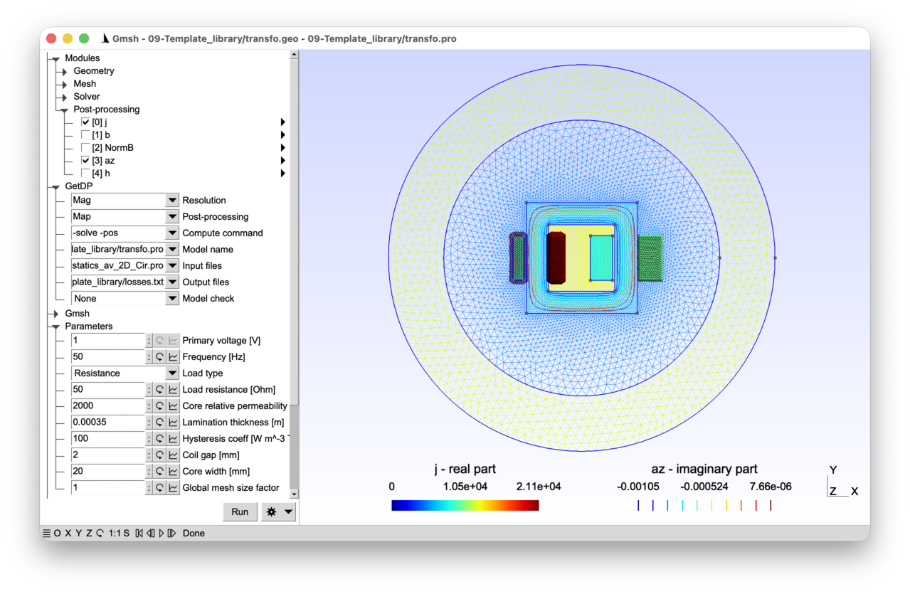
2.9.1 Features 
- Two electrically independent, magnetically coupled circuits
- Stranded coils with number of turns, cross-section area and go/return sides
- Homogenized laminated ferromagnetic core
- Use of a generic template formulation library
See the comments in transfo.pro and transfo.geo for details.
2.9.2 Running the tutorial 
On the command line:
> gmsh transfo.geo -2
> getdp transfo.pro -solve Mag -pos Map
Interactively with Gmsh: open transfo.pro with “File->Open”, then press “Run”.
2.9.3 Contents 
File transfo_common.pro 
// Parameters shared by Gmsh and GetDP: core and coil dimensions.

mm = 1e-3;
wCore = 100 * mm;
hCore = 100 * mm;
wCoil1 = 10 * mm;
hCoil1 = 40 * mm;
wCoil2 = 20 * mm;
hCoil2 = 40 * mm;

DefineConstant[
  thickCore = {30, Min 5, Max 60, Step 0.1,
    Name "Parameters/Core thickness [mm]", Visible 0}
  gapCoil = {2, Min 0.5, Max 7.5, Step 0.1,
    Name "Parameters/Coil gap [mm]"}
  wCoreLeg = {20, Min 10, Max 27, Step 0.1,
    Name "Parameters/Core width [mm]"}
];

thickCore = thickCore * mm;
gapCoil = gapCoil * mm;
wCoreLeg = wCoreLeg * mm;

// Inner and outer radii for the infinite shell Jacobian (see tutorial 3),
// chosen to be large enough to enclose the full geometry:
r = Max[(wCore + 2 * gapCoil + wCoil1 + wCoil2) / 2, hCore / 2];
JacRadiusInt = r * Sqrt[2] + 30 * mm;
JacRadiusExt = JacRadiusInt + 50 * mm;
File transfo.geo 
// Gmsh script describing the geometry of a single-phase transformer: a
// ferromagnetic core with a primary winding (two coil sides) and a secondary
// winding (two coil sides), surrounded by an air region with an infinite shell
// for the unbounded domain (see tutorial 3).

SetFactory("OpenCASCADE");

Include "transfo_common.pro";

// The core is is created by subtracting the inner rectangle (the window) from
// the outer rectangle:
Rectangle(1) = {-wCore / 2, -hCore / 2, 0,
  wCore, hCore};
Rectangle(2) = {-wCore / 2 + wCoreLeg, -hCore / 2 + wCoreLeg, 0,
  wCore - 2 * wCoreLeg, hCore - 2 * wCoreLeg};

// Primary winding: two coil sides (minus and plus) on either side of the left
// core leg. "Coil1M" carries the current in the -z direction and "Coil1P" in
// the +z direction (the go and return paths of the same winding):
Rectangle(3) = {-wCore / 2 - gapCoil - wCoil1, -hCoil1 / 2, 0,
  wCoil1, hCoil1};
Rectangle(4) = {-wCore / 2 + wCoreLeg + gapCoil, -hCoil1 / 2, 0,
  wCoil1, hCoil1};

// Secondary winding: two coil sides on either side of the right core leg:
Rectangle(5) = {wCore / 2 - wCoreLeg - gapCoil - wCoil2, -hCoil2 / 2, 0,
  wCoil2, hCoil1};
Rectangle(6) = {wCore / 2 + gapCoil, -hCoil2 / 2, 0,
  wCoil2, hCoil2};

// Air region (disk) and infinite ring:
Disk(7) = {0, 0, 0, JacRadiusInt};
Disk(8) = {0, 0, 0, JacRadiusExt};

// Make all overlapping surfaces conformal (see tutorial 3):
Coherence;

// Use the "Closest" command to retrieve the regions that were split by the
// boolean operation in "Coherence":
airinf() = Closest {JacRadiusInt + 1e-6, 0, 0} { Surface{:}; };
core() = Closest {wCore / 2 - 1e-6, 0, 0} { Surface{:}; };

// The air region is everything except the infinite shell, the core and the
// coils:
air() = Surface{:};
air() -= {airinf(0), core(0), 3, 4, 5, 6};

bnd() = CombinedBoundary{ Surface{:}; };

DefineConstant[
  s = {1, Min 0.1, Max 10, Step 0.1,
    Name "Parameters/}Global mesh size factor"}
];

MeshSize{:} = 2 * mm * s;
MeshSize{ PointsOf{ Surface{airinf(0)}; } } = 8 * mm * s;

Physical Surface("Air", 1) = air();
Physical Surface("AirInf", 2) = airinf(0);
Physical Surface("Coil1M", 3) = 3;
Physical Surface("Coil1P", 4) = 4;
Physical Surface("Coil2M", 5) = 5;
Physical Surface("Coil2P", 6) = 6;
Physical Surface("Core", 7) = core(0);
Physical Curve("Bnd", 10) = bnd();
File transfo.pro 
// This tutorial models a single-phase transformer with two windings (primary
// and secondary) wound around a laminated ferromagnetic core, using a
// frequency-domain magneto-quasistatic a-v formulation coupled with two
// external circuits.
//
// Whereas previous tutorials built the complete formulation, function spaces,
// resolution and post-processing from scratch, this tutorial illustrates the
// use of a generic template library ("Lib_Magnetoquasistatics_av_2D_Cir.pro").
// The library provides a ready-made a-v formulation that handles massive
// conductors, stranded coils, nonlinear materials, permanent magnets, impedance
// boundary conditions, and circuit coupling. The user only needs to define the
// physical and abstract groups, the material properties, the constraints, and a
// few configuration variables -- the rest is taken care of by the library.
//
// The main new modeling concepts introduced in the tutorial are the modeling of
// stranded coils and of the ferromagnetic laminations in the core.
//
// Unlike the massive (solid) conductors of tutorials 7 and 8, where eddy
// currents are resolved inside the conductor cross-section, a stranded coil is
// modeled as a homogenized region carrying a uniform current density
//
//   j = Ns / Sc * I * z_hat,
//
// where "Ns" is the number of turns, "Sc" the cross-sectional area of the
// winding, "I" the total current (the same in each turn), and "z_hat" the unit
// vector along the conductor direction. This approximation is valid when the
// coil consists of a large number of turns in series with each other (so that
// the each turn carries the same current), where each individual turn is thin
// compared to the skin depth (so that the current distribution within each turn
// is essentially uniform).

// Each winding consists of two coil sides (the "go" and "return" halves of the
// same winding), modeled as separate regions with opposite current
// directions. The two windings are connected to two independent circuits:
//
//   Circuit 1 (primary):   voltage source E_in -> Coil_1_M -> Coil_1_P
//   Circuit 2 (secondary): Coil_2_M -> Coil_2_P -> load impedance Z_out
//
// The magnetic coupling between the two circuits occurs through the shared
// magnetic flux in the core -- there is no explicit electrical connection
// between them, i.e., they are galvanically isolated. The load connected at the
// terminals of the secondary can be a resistance, an inductance, or a
// capacitance, selected at runtime through a "DefineConstant" parameter.
//
// We define an effective complex reluctivity "nu = nu_r + i * nu_i = nu_r + i *
// (nu_H + nu_EC)" to model the hysteresis and eddy current losses in the
// laminated ferromagnetic core. The imaginary part of the reluctivity
// introduces a dissipative contribution "(1/2) * omega * (nu_H + nu_EC) *
// |B_peak|^2" per unit volume.
//
//  - Hysteresis losses: Each magnetisation cycle dissipates approximately
//
//      p_H = kh * |B_peak|^2,
//
//    with an empirical coefficient kh. Matching with "(1/2) * omega * nu_H *
//    |B_peak|^2p_H" gives
//
//      nu_H = kh / Pi.
//
//    This equivalent reluctivity is frequency-independent and hysteresis losses
//    p_H are proportional to the frequency "f" (through "omega").
//
//  - Eddy current losses: in a lamination of thickness "d" and bulk
//    conductivity "sigma_iron", eddy-current losses are approximately given by
//    (see e.g. J. Gyselinck et al., "Calculation of eddy currents and
//    associated losses in electrical steel laminations", IEEE Transactions on
//    Magnetics, 35(3), 1191-1194, 1999):
//
//      p_EC = (1/2) * sigma_iron * (d * omega * |B_peak|)^2 / 12.
//
//    Matching with "(1/2) * omega * nu_EC * |B_peak|^2" gives
//
//      nu_EC = sigma_iron * omega * d^2 / 12.
//
//    This equivalent reluctivity is proportional to the frequency, and
//    eddy-current losses "p_EC" thus scale as "f^2".

Include "transfo_common.pro";

Group {
  // Physical regions:
  Air = Region[ 1 ];
  AirInf = Region[ 2 ];
  Coil_1_M = Region[ 3 ];
  Coil_1_P = Region[ 4 ];
  Coil_2_M = Region[ 5 ];
  Coil_2_P = Region[ 6 ];
  Coil_1 = Region[ {Coil_1_M, Coil_1_P} ];
  Coil_2 = Region[ {Coil_2_M, Coil_2_P} ];
  Coils = Region[ {Coil_1, Coil_2} ];
  Core = Region[ 7 ];
  Bnd = Region[ 10 ]; // exterior boundary

  // Abstract regions expected by the template library. The role of each group
  // is documented in "Lib_Magnetoquasistatics_av_2D_Cir.pro":
  //  - "Vol_Mag": full magnetic domain
  //  - "Vol_S_Mag": stranded conductors (windings with Ns turns)
  //  - "Vol_Inf_Mag": region with infinite shell transformation
  Vol_Mag = Region[ {Air, AirInf, Core, Coils} ];
  Vol_S_Mag = Region[ Coils ];
  Vol_Inf_Mag = Region[ AirInf ];

  // Circuit regions (fictitious, as in tutorial 8): the voltage source on the
  // primary side and the load impedance on the secondary side:
  E_in = Region[ 100 ];
  Z_out = Region[ 102 ];

  // Abstract circuit regions expected by the library:
  //  - "Source_Cir": all voltage and current sources
  //  - "Resistance_Cir": all resistors
  //  - "Inductance_Cir": all inductors
  //  - "Capacitance_Cir": all capacitors
  Source_Cir = Region[ {E_in} ];
  DefineConstant[
    LoadType = {0, Choices {0="Resistance", 1="Inductance", 2="Capacitance"},
      Name "Parameters/2Load type"}
  ];
  // "LoadType" determines which abstract circuit group "Z_out" belongs to.
  // Each group has a different constitutive relation in the library formulation
  // (see tutorial 8 for the lumped element GlobalTerms):
  If(LoadType == 0)
    Resistance_Cir = Region[ {Z_out} ];
  ElseIf(LoadType == 1)
    Inductance_Cir = Region[ {Z_out} ];
  Else
    Capacitance_Cir = Region[ {Z_out} ];
  EndIf
}

Function {
  DefineConstant[
    Voltage = {1, Min 1e-3, Max 10,
      Name "Parameters/0Primary voltage [V]"}
    f = {50, Min 0, Max 1e3, Step 1,
      Name "Parameters/1Frequency [Hz]"}
    Rval = {50, Min 1e-3, Max 50, Step 0.25, Visible (LoadType == 0),
      Name "Parameters/3Load resistance [Ohm]"}
    Lval = {1e-6, Min 1e-9, Max 0.1, Step 1e-3, Visible (LoadType == 1),
      Name "Parameters/3Load inductance [H]"}
    Cval = {1e-6, Min 1e-9, Max 0.1, Step 1e-4, Visible (LoadType == 2),
      Name "Parameters/3Load capacitance [F]"}
    // Typical values for grain-oriented Si-steel (M3, 0.35 mm laminations):
    murCore = {2000, Min 1, Max 10000, Step 1,
      Name "Parameters/4Core relative permeability"}
    dlam = {0.35e-3, Min 0.1e-3, Max 1e-3, Step 0.05e-3,
      Name "Parameters/5Lamination thickness [m]"}
    kh = {100, Min 10, Max 500, Step 10,
      Name "Parameters/6Hysteresis coeff [W m^-3 T^-2 s]"}
  ];

  mu0 = 4e-7 * Pi;
  nu[ Air ] = 1 / mu0;
  nu[ AirInf ] = 1 / mu0;

  // Homogenized effective reluctivity to take into account losses in the
  // laminated ferromagnetic core:
  nu_r = 1 / (murCore * mu0);
  sigma_iron = 2e6;
  nu_i = kh / Pi + sigma_iron * (2 * Pi * f) * dlam^2 / 12;
  nu[ Core ] = Complex[nu_r, nu_i];

  // Stranded coil parameters expected by the library:
  //  - "Ns[]": number of turns in each winding
  //  - "Sc[]": cross-sectional area of each coil side. "SurfaceArea[]" is a
  //    built-in GetDP function that returns the area of the region on which it
  //    is evaluated
  Ns[ Coil_1 ] = 100;
  Ns[ Coil_2 ] = 200;
  Sc[ Coil_1_M ] = SurfaceArea[];
  Sc[ Coil_1_P ] = SurfaceArea[];
  Sc[ Coil_2_M ] = SurfaceArea[];
  Sc[ Coil_2_P ] = SurfaceArea[];
  nu[ Coils ] = 1 / mu0;
  // The conductivity of the stranded coils enters the Joule losses calculation
  // in the library (via the DC resistance term "Ns^2 / (sigma * Sc^2)"):
  sigma[ Coils ] = 5.8e7;

  // Geometrical coefficient in all the regions with global voltages and
  // currents, to specify the out-of-plane thickness and control the current
  // direction (as in tutorials 7 and 8):
  CoefGeo[ Coil_1_M ] = -1 * thickCore;
  CoefGeo[ Coil_1_P ] = 1 * thickCore;
  CoefGeo[ Coil_2_M ] = -1 * thickCore;
  CoefGeo[ Coil_2_P ] = 1 * thickCore;
  CoefGeo[ Core ] = thickCore;

  // Lumped circuit element parameters (as in tutorial 8):
  Resistance[ Z_out ] = Rval;
  Inductance[ Z_out ] = Lval;
  Capacitance[ Z_out ] = Cval;
}

Constraint {
  // Homogeneous Dirichlet condition on the vector potential at infinity:
  { Name a_Mag_2D;
    Case {
      { Region Bnd; Value 0; }
    }
  }

  // No imposed current or voltage on the FE coils (determined by the circuit):
  { Name Current_Mag_2D;
    Case {
    }
  }
  { Name Voltage_Mag_2D;
    Case {
    }
  }

  // No imposed current on circuit elements (the inductor initial condition is
  // only needed in the time domain, which is not used here):
  { Name Current_Cir ;
    Case {
    }
  }

  // Imposed voltage on the primary voltage source (as in tutorial 8):
  { Name Voltage_Cir ;
    Case {
      { Region E_in; Value Voltage; TimeFunction F_Cos_wt_p[]{2 * Pi * f, 0}; }
    }
  }

  // The circuit topology uses two independent circuits. "Circuit_1" and
  // "Circuit_2" define separate connected networks, each with its own set of
  // circuit nodes (the node numbers are local to each case). This allows
  // modeling magnetically coupled but electrically isolated windings -- the
  // coupling between the two circuits happens through the shared magnetic flux
  // in the finite element model, not through any electrical connection.
  { Name ElectricalCircuit ; Type Network ;
    Case Circuit_1 {
      // Primary circuit: voltage source driving the primary winding. The two
      // coil sides are connected in series (nodes 1 -> 2 -> 3 -> back to 1):
      { Region E_in; Branch {1, 2}; }
      { Region Coil_1_M; Branch {2, 3} ; }
      { Region Coil_1_P; Branch {3, 1} ; }
    }
    Case Circuit_2 {
      // Secondary circuit: the secondary winding drives the load. Note that the
      // secondary has no external source -- the voltage is induced by the
      // time-varying flux from the primary:
      { Region Coil_2_M; Branch {1, 2} ; }
      { Region Coil_2_P; Branch {2, 3} ; }
      { Region Z_out; Branch {3, 1}; }
    }
  }
}

// Configuration of the template library. The following variables are read by
// "Lib_Magnetoquasistatics_av_2D_Cir.pro" to select the analysis type and
// enable the appropriate features (the full list of configuration variables is
// documented at the beginning of the library file):
CircuitCoupling = 1;
AnalysisType = 2; // frequency-domain
CoefPower = 0.5; // peak-valued phasors
Freq = f;
Include "Lib_Magnetoquasistatics_av_2D_Cir.pro";

// The library is made generic through three GetDP declaration commands:
//  - "DefineConstant[]": defines a constant only if it has not already been
//    defined. The library uses it to set default values for all its
//    configuration variables (AnalysisType, Axisymmetric, Freq, etc.). If the
//    user sets a variable before the "Include", it takes precedence; otherwise
//    the library's default applies.
//  - "DefineGroup[]": similarly, declares a group only if it does not already
//    exist. The library declares all the abstract groups it knows about
//    (Vol_Mag, Vol_C_Mag, Vol_S_Mag, Vol_NL_Mag, Vol_M_Mag, etc.) with empty
//    defaults. The user populates only the groups relevant to the problem at
//    hand; unused groups remain empty and the corresponding terms in the
//    formulation are silently skipped (since an integral over an empty region
//    contributes nothing).
//  - "DefineFunction[]": declares a function only if it does not already exist.
//    The library declares all the material functions it may use (nu[], sigma[],
//    br[], js0[], etc.); the user defines only those needed for the problem.
//
// This "define-if-absent" mechanism allows a single library file to handle
// magnetostatics, eddy currents, permanent magnets, stranded coils, circuit
// coupling, nonlinear materials and impedance boundary conditions -- all
// controlled by which groups and functions the user chooses to populate before
// the "Include".

// The PostOperation is specific to this model: the library provides the
// PostProcessing (with quantities like "az", "b", "j", "U", "I", "NormU",
// "NormI", etc.), but the user decides what to print and where.
PostOperation {
  { Name Map; NameOfPostProcessing Mag;
    Operation {
      Print[ j, OnElementsOf Vol_Mag, Format Gmsh, File "j.pos" ];
      Print[ b, OnElementsOf Vol_Mag, Format Gmsh, File "b.pos" ];
      Print[ NormB, OnElementsOf Vol_Mag, Format Gmsh, File "normb.pos" ];
      Print[ az, OnElementsOf Vol_Mag, Format Gmsh, File "az.pos" ];
      Print[ h, OnElementsOf Core, Format Gmsh, File "h.pos" ];

      Echo[ "E_in", Format Table, File "UI.txt" ];
      Print[ U, OnRegion E_in, Format FrequencyTable, File > "UI.txt"];
      Print[ I, OnRegion E_in, Format FrequencyTable, File > "UI.txt"];
      Echo[ "Z_out", Format Table, File > "UI.txt" ];
      Print[ U, OnRegion Z_out, Format FrequencyTable, File > "UI.txt"];
      Print[ I, OnRegion Z_out, Format FrequencyTable, File > "UI.txt"];

      // The "{0}" suffix after the parameter name selects only the first
      // component to be sent to Gmsh (instead of both the real and imaginary
      // part, as all values are complex):
      Print[ NormU, OnRegion E_in, Format Table, File "",
        SendToServer "}Output/0|V_in| [V]"{0} ];
      Print[ NormI, OnRegion E_in, Format Table, File "",
        SendToServer "}Output/1|I_in| [A]"{0} ];
      Print[ NormU, OnRegion Z_out, Format Table, File "",
        SendToServer "}Output/2|V_out| [V]"{0} ];
      Print[ NormI, OnRegion Z_out, Format Table, File "",
        SendToServer "}Output/3|I_out| [A]"{0} ];

      // To interactively plot the exterior characteristic |V_out|(|I_out|) with
      // Gmsh, click the "Loop" arrow button next to the load value in the
      // "Parameters" menu (this sweeps the load over its allowed range), then
      // press "Run". Click the "Draw" graph button next to |I_out| and select
      // e.g. "Top left -> X", then click the "Draw" graph button next to
      // |V_out| and select "Top left -> Y" -- you can do this while the sweep
      // is still running to watch the curve build up live. The two quantities
      // are then plotted against each other in a graph anchored to the top-left
      // corner of the Gmsh window, with |I_out| on the X axis and |V_out| on
      // the Y axis.

      Print[ JouleLosses[Vol_Mag], OnGlobal, Format Table,
        File "losses.txt", SendToServer "}Output/p_Joule [W m^-3]"{0} ];
      Print[ HarmonicMagneticLosses[Vol_Mag], OnGlobal, Format Table,
        File > "losses.txt", SendToServer "}Output/p_H+EC [W m^-3]"{0} ];
    }
  }
}
File Lib_Magnetoquasistatics_av_2D_Cir.pro 
// Lib_Magnetoquasistatics_av_2D_Cir.pro
//
// Template library for 2D magneto-quasistatic problems in terms of the magnetic
// vector potential "a" and the electric scalar potential "v", with optional
// circuit coupling.

// Default definitions of constants, groups and functions that can (should) be
// redefined from outside the template:

DefineConstant[
  AnalysisType = 1, // static (0), time-domain (1) or frequency-domain (2)
  Axisymmetric = 0, // axisymmetric model?
  CircuitCoupling = 0, // consider coupling with external electric circuit
  NewtonRaphson = 1, // Newton-Raphson or Picard method for nonlinear iterations
  CoefPower = 1, // power calculation coefficient (0.5 for peak-valued phasors)
  Freq = 50, // frequency (for harmonic simulations)
  TimeInit = 0, // initial time (for time-domain simulations)
  TimeFinal = 1/50, // final time (for time-domain simulations)
  DeltaTime = 1/500, // time step (for time-domain simulations)
  FEOrder = 1, // finite element order
  JacRadiusInt = 0, // interior radius for spherical shell (Vol_Inf_Mag)
  JacRadiusExt = 0, // exterior radius of spherical shell (Vol_Inf_Mag)
  JacCenterX = 0, // x-coordinate of center of Vol_Inf_Mag
  JacCenterY = 0, // y-coordinate of center of Vol_Inf_Mag
  JacCenterZ = 0, // z-coordinate of center of Vol_Inf_Mag
  NLTolAbs = 1e-10, // absolute tolerance on residual for nonlinear iterations
  NLTolRel = 1e-6, // relative tolerance on residual for nonlinear iterations
  NLIterMax = 20 // maximum number of nonlinear iterations
];

Group {
  DefineGroup[
    // The full magnetic domain:
    Vol_Mag,

    // Subsets of Vol_Mag:
    Vol_C_Mag, // massive conductors
    Vol_S_Mag, // stranded conductors
    Vol_S0_Mag, // stranded conductors with imposed current density js0
    Vol_NL_Mag, // nonlinear magnetic materials
    Vol_V_Mag, // moving massive conducting parts (with invariant mesh)
    Vol_M_Mag, // permanent magnets
    Vol_Inf_Mag, // annulus where an infinite shell transformation is applied

    // Boundaries:
    Sur_Neu_Mag, // non-homogeneous Neumann BC (flux tube with n x h = nxh[])
    Sur_Imped_Mag // conductors approximated by an impedance (non-meshed)
  ];
  If(CircuitCoupling)
    DefineGroup[
      Source_Cir, // voltage and current sources
      Resistance_Cir, // resistors
      Inductance_Cir, // inductors
      Capacitance_Cir // capacitors
    ];
  EndIf
}

Function {
  DefineFunction[
    nu, // reluctivity (in Vol_Mag)
    sigma, // conductivity (in Vol_C_Mag and Vol_S_Mag)
    br, // remanent magnetic flux density (in Vol_M_Mag)
    js0, // source current density (in Vol_S0_Mag)
    dhdb, // Jacobian for Newton-Raphson method (in Vol_NL_Mag)
    nxh, // n x magnetic field (on Sur_Neu_Mag)
    Velocity, // velocity of moving part (in Vol_V_Mag)
    Ns, // number of turns (in Vol_S_Mag)
    Sc, // cross-section of windings (in Vol_S_Mag)
    CoefGeo, // thickness (2D) or 2 * Pi (axisymmetric) geometrical coefficient
             // (in Vol_Mag); negative to set positive current along -z
    Ysur // surface admittance (on Sur_Imped_Mag)
  ];
  If(CircuitCoupling)
    DefineFunction[
      Resistance, // lumped resistance values
      Inductance, // lumped inductance values
      Capacitance // lumped capacitance values
    ];
  EndIf
}

// End of default definitions.

Jacobian {
  { Name JacVol_Mag;
    Case {
      If(Axisymmetric)
        { Region Vol_Inf_Mag;
          Jacobian VolAxiSquSphShell{JacRadiusInt, JacRadiusExt,
                                     JacCenterX, JacCenterY, JacCenterZ}; }
        { Region All; Jacobian VolAxiSqu; }
      Else
        { Region Vol_Inf_Mag;
          Jacobian VolSphShell{JacRadiusInt, JacRadiusExt,
                               JacCenterX, JacCenterY, JacCenterZ}; }
        { Region All; Jacobian Vol; }
      EndIf
    }
  }
  { Name JacSur_Mag;
    Case {
      If(Axisymmetric)
        { Region All; Jacobian SurAxi; }
      Else
        { Region All; Jacobian Sur; }
      EndIf
    }
  }
}

Integration {
  { Name Int_Mag;
    Case {
      { Type Gauss;
        Case {
          { GeoElement Point; NumberOfPoints  1; }
          { GeoElement Line; NumberOfPoints (FEOrder == 1) ? 2 : 4; }
          { GeoElement Triangle; NumberOfPoints (FEOrder == 1) ? 3 : 6; }
          { GeoElement Quadrangle; NumberOfPoints (FEOrder == 1) ? 4 : 16; }
        }
      }
    }
  }
}

Group{
  Dom_Hcurl_a_Mag_2D = Region[ {Vol_Mag, Sur_Neu_Mag, Sur_Imped_Mag} ];
  Dom_Hcurl_u_Mag_2D = Region[ {Vol_C_Mag, Sur_Imped_Mag} ];
  If(CircuitCoupling)
    Dom_Cir = Region[ {Source_Cir, Resistance_Cir, Inductance_Cir, Capacitance_Cir} ];
  EndIf
}

FunctionSpace {
  // Magnetic vector potential
  { Name Hcurl_a_Mag_2D; Type Form1P;
    BasisFunction {
      { Name se; NameOfCoef ae; Function BF_PerpendicularEdge;
        Support Dom_Hcurl_a_Mag_2D; Entity NodesOf[All]; }
      If(FEOrder == 2)
        { Name se2; NameOfCoef ae2; Function BF_PerpendicularEdge_2E;
          Support Dom_Hcurl_a_Mag_2D; Entity EdgesOf[All]; }
      EndIf
    }
    Constraint {
      { NameOfCoef ae; EntityType NodesOf; NameOfConstraint a_Mag_2D; }
      If(FEOrder == 2)
        { NameOfCoef ae2; EntityType EdgesOf; NameOfConstraint a0_Mag_2D; }
      EndIf
    }
  }

  // Gradient of scalar electric potential
  { Name Hcurl_u_Mag_2D; Type Form1P;
    BasisFunction {
      { Name sr; NameOfCoef ur; Function BF_RegionZ;
        Support Dom_Hcurl_u_Mag_2D; Entity Dom_Hcurl_u_Mag_2D; }
    }
    GlobalQuantity {
      { Name Voltage; Type AliasOf; NameOfCoef ur; }
      { Name Current; Type AssociatedWith; NameOfCoef ur; }
    }
    Constraint {
      { NameOfCoef Voltage; EntityType Region; NameOfConstraint Voltage_Mag_2D; }
      { NameOfCoef Current; EntityType Region; NameOfConstraint Current_Mag_2D; }
    }
  }

  // Current in stranded coils
  { Name Hregion_i_Mag_2D; Type Vector;
    BasisFunction {
      { Name sr; NameOfCoef ir; Function BF_RegionZ;
        Support Vol_S_Mag; Entity Vol_S_Mag; }
    }
    GlobalQuantity {
      { Name Current; Type AliasOf; NameOfCoef ir; }
      { Name Voltage; Type AssociatedWith; NameOfCoef ir; }
    }
    Constraint {
      { NameOfCoef Voltage; EntityType Region; NameOfConstraint Voltage_Mag_2D; }
      { NameOfCoef Current; EntityType Region; NameOfConstraint Current_Mag_2D; }
    }
  }

  If(CircuitCoupling)
    // Current in lumped circuit elements
    { Name Hregion_i_Cir; Type Scalar;
      BasisFunction {
        { Name sr; NameOfCoef ir; Function BF_Region;
          Support Dom_Cir; Entity Dom_Cir; }
      }
      GlobalQuantity {
        { Name Current; Type AliasOf; NameOfCoef ir; }
        { Name Voltage; Type AssociatedWith; NameOfCoef ir; }
      }
      Constraint {
        { NameOfCoef Voltage; EntityType Region; NameOfConstraint Voltage_Cir; }
        { NameOfCoef Current; EntityType Region; NameOfConstraint Current_Cir; }
      }
    }
  EndIf
}

Group{
  // all linear materials
  Vol_L_Mag = Region[ {Vol_Mag, -Vol_NL_Mag} ];
}

Formulation {
  { Name Magnetoquasistatics_av_2D; Type FemEquation;
    Quantity {
      { Name a; Type Local; NameOfSpace Hcurl_a_Mag_2D; }
      { Name ir; Type Local; NameOfSpace Hregion_i_Mag_2D; }
      { Name Us; Type Global; NameOfSpace Hregion_i_Mag_2D [Voltage]; }
      { Name Is; Type Global; NameOfSpace Hregion_i_Mag_2D [Current]; }
      If(AnalysisType > 0)
        { Name ur; Type Local; NameOfSpace Hcurl_u_Mag_2D; }
        { Name U; Type Global; NameOfSpace Hcurl_u_Mag_2D [Voltage]; }
        { Name I; Type Global; NameOfSpace Hcurl_u_Mag_2D [Current]; }
        If(CircuitCoupling)
          { Name Uz; Type Global; NameOfSpace Hregion_i_Cir [Voltage]; }
          { Name Iz; Type Global; NameOfSpace Hregion_i_Cir [Current]; }
        EndIf
      EndIf
    }
    Equation {
      Integral { [ nu[] * Dof{d a} , {d a} ];
        In Vol_L_Mag; Jacobian JacVol_Mag; Integration Int_Mag; }

      If(NewtonRaphson)
        Integral { [ nu[{d a}] * {d a} , {d a} ];
          In Vol_NL_Mag; Jacobian JacVol_Mag; Integration Int_Mag; }
        Integral { [ dhdb[{d a}] * Dof{d a} , {d a} ];
          In Vol_NL_Mag; Jacobian JacVol_Mag; Integration Int_Mag; }
        Integral { [ - dhdb[{d a}] * {d a} , {d a} ];
          In Vol_NL_Mag; Jacobian JacVol_Mag; Integration Int_Mag; }
      Else
        Integral { [ nu[{d a}] * Dof{d a}, {d a} ];
          In Vol_NL_Mag; Jacobian JacVol_Mag; Integration Int_Mag; }
      EndIf

      Integral { [ - nu[] * br[] , {d a} ];
        In Vol_M_Mag; Jacobian JacVol_Mag; Integration Int_Mag; }

      Integral { [ - js0[] , {a} ];
        In Vol_S0_Mag; Jacobian JacVol_Mag; Integration Int_Mag; }
      Integral { [ - Ns[] / Sc[] * Sign[CoefGeo[]] * Dof{ir} , {a} ];
        In Vol_S_Mag; Jacobian JacVol_Mag; Integration Int_Mag; }

      Integral { [ Ns[]^2 / Sc[]^2 / sigma[] * Sign[CoefGeo[]] * Dof{ir} , {ir} ];
        In Vol_S_Mag; Jacobian JacVol_Mag; Integration Int_Mag; }
      GlobalTerm { [ Dof{Us} / CoefGeo[] , {Is} ]; In Vol_S_Mag; }

      Integral { [ nxh[] , {a} ];
        In Sur_Neu_Mag; Jacobian JacSur_Mag; Integration Int_Mag; }

      If(AnalysisType > 0)
        Integral { DtDof [ sigma[] * Dof{a} , {a} ];
          In Vol_C_Mag; Jacobian JacVol_Mag; Integration Int_Mag; }
        Integral { [ sigma[] * Dof{ur} / CoefGeo[] , {a} ];
          In Vol_C_Mag; Jacobian JacVol_Mag; Integration Int_Mag; }

        Integral { [ - sigma[] * (Velocity[] /\ Dof{d a}) , {a} ];
          In Vol_V_Mag; Jacobian JacVol_Mag; Integration Int_Mag; }

        Integral { DtDof [  Ysur[] * Dof{a} , {a} ];
          In Sur_Imped_Mag; Jacobian JacSur_Mag; Integration Int_Mag; }
        Integral { [ Ysur[] * Dof{ur} / CoefGeo[] , {a} ];
          In Sur_Imped_Mag; Jacobian JacSur_Mag; Integration Int_Mag; }

        Integral { DtDof [ sigma[] * Dof{a} , {ur} ];
          In Vol_C_Mag; Jacobian JacVol_Mag; Integration Int_Mag; }
        Integral { [ sigma[] * Dof{ur} / CoefGeo[] , {ur} ];
          In Vol_C_Mag; Jacobian JacVol_Mag; Integration Int_Mag; }
        GlobalTerm { [ Dof{I} *(CoefGeo[]/Fabs[CoefGeo[]]) , {U} ]; In Vol_C_Mag; }

        Integral { DtDof [ Ysur[] * Dof{a} , {ur} ];
          In Sur_Imped_Mag; Jacobian JacSur_Mag; Integration Int_Mag; }
        Integral { [ Ysur[] * Dof{ur} / CoefGeo[] , {ur} ];
          In Sur_Imped_Mag; Jacobian JacSur_Mag; Integration Int_Mag; }
        GlobalTerm { [ Dof{I} * (CoefGeo[] / Fabs[CoefGeo[]]) , {U} ]; In Sur_Imped_Mag; }

        Integral { DtDof [ Ns[] / Sc[] * Dof{a} , {ir} ];
          In Vol_S_Mag; Jacobian JacVol_Mag; Integration Int_Mag; }

        If(CircuitCoupling)
          GlobalTerm { NeverDt[ Dof{Uz} , {Iz} ]; In Resistance_Cir; }
          GlobalTerm { NeverDt[ Resistance[{Uz}] * Dof{Iz} , {Iz} ]; In Resistance_Cir; }

          GlobalTerm { [ Dof{Uz} , {Iz} ]; In Inductance_Cir; }
          GlobalTerm { DtDof [ Inductance[] * Dof{Iz} , {Iz} ]; In Inductance_Cir; }

          GlobalTerm { NeverDt[ Dof{Iz} , {Iz} ]; In Capacitance_Cir; }
          GlobalTerm { DtDof [ Capacitance[] * Dof{Uz} , {Iz} ]; In Capacitance_Cir; }

          GlobalTerm { [ 0. * Dof{Iz} , {Iz} ]; In Source_Cir; }

          GlobalEquation {
            Type Network; NameOfConstraint ElectricalCircuit;
            { Node {I};  Loop {U};  Equation {I};  In Vol_C_Mag; }
            { Node {Is}; Loop {Us}; Equation {Us}; In Vol_S_Mag; }
            { Node {Iz}; Loop {Uz}; Equation {Uz}; In Dom_Cir; }
          }
        EndIf
      EndIf
    }
  }
}

Resolution {
  { Name Mag;
    System {
      { Name A; NameOfFormulation Magnetoquasistatics_av_2D;
        If(AnalysisType == 2)
          Type ComplexValue; Frequency Freq;
        EndIf
      }
    }
    Operation {
      If(AnalysisType == 0 || AnalysisType == 2)
        Generate[A]; Solve[A]; SaveSolution[A];
      Else
        InitSolution[A];
        TimeLoopTheta[TimeInit, TimeFinal, DeltaTime, 1.]{
          Generate[A]; Solve[A];
          If(NbrRegions[Vol_NL_Mag])
            Generate[A]; GetResidual[A, $res0];
            Evaluate[ $res = $res0, $iter = 0 ];
            Print[{$iter, $res, $res / $res0},
              Format "Residual %03g: abs %14.12e rel %14.12e"];
            While[$res > NLTolAbs && $res / $res0 > NLTolRel &&
                  $res / $res0 <= 1 && $iter < NLIterMax]{
              Solve[A]; Generate[A]; GetResidual[A, $res];
              Evaluate[ $iter = $iter + 1 ];
              Print[{$iter, $res, $res / $res0},
                Format "Residual %03g: abs %14.12e rel %14.12e"];
            }
          EndIf
          SaveSolution[A];
        }
      EndIf
    }
  }
}

PostProcessing {
  { Name Mag; NameOfFormulation Magnetoquasistatics_av_2D;
    Quantity {
      { Name a; Value {
          Term { [ {a} ]; In Vol_Mag; Jacobian JacVol_Mag; }
        }
      }
      { Name az; Value {
          Term { [ CompZ[{a}] ]; In Vol_Mag; Jacobian JacVol_Mag; }
        }
      }
      { Name xaz; Value {
          Term { [ X[] * CompZ[{a}] ]; In Vol_Mag; Jacobian JacVol_Mag; }
        }
      }
      { Name b; Value {
          Term { [ {d a} ]; In Vol_Mag; Jacobian JacVol_Mag; }
        }
      }
      { Name NormB; Value {
          Term { [ Norm[{d a}] ]; In Vol_Mag; Jacobian JacVol_Mag; }
        }
      }
      { Name h; Value {
          Term { [ nu[] * {d a} ]; In Vol_L_Mag; Jacobian JacVol_Mag; }
          Term { [ nu[{d a}] * {d a} ]; In Vol_NL_Mag; Jacobian JacVol_Mag; }
          Term { [ -nu[] * br[] ]; In Vol_M_Mag; Jacobian JacVol_Mag; }
        }
      }
      { Name j; Value {
          If(AnalysisType > 0)
            Term { [ -sigma[] * (Dt[{a}] + {ur} / CoefGeo[]) ];
              In Vol_C_Mag; Jacobian JacVol_Mag; }
            // Current density in A/m
            Term { [ -Ysur[] * (Dt[{a}] + {ur} / CoefGeo[]) ];
              In Sur_Imped_Mag; Jacobian JacSur_Mag; }
          EndIf
          Term { [ js0[] ];
            In Vol_S0_Mag; Jacobian JacVol_Mag; }
          Term { [ Ns[] / Sc[] * Sign[CoefGeo[]] * {ir} ];
            In Vol_S_Mag; Jacobian JacVol_Mag; }
          Term { [ Vector[0, 0, 0] ];
            In Vol_Mag; Jacobian JacVol_Mag; }
        }
      }
      { Name U; Value {
          If(AnalysisType > 0)
            Term { [ {U} ]; In Vol_C_Mag; }
            If(CircuitCoupling)
              Term { [ {Uz} ]; In Dom_Cir; }
            EndIf
          EndIf
          Term { [ {Us} ]; In Vol_S_Mag; }
        }
      }
      { Name I; Value {
          If(AnalysisType > 0)
            Term { [ {I} ]; In Vol_C_Mag; }
            If(CircuitCoupling)
              Term { [ {Iz} ]; In Dom_Cir; }
            EndIf
          EndIf
          Term { [ {Is} ]; In Vol_S_Mag; }
        }
      }
      { Name NormU; Value {
          If(AnalysisType > 0)
            Term { [ Norm[{U}] ]; In Vol_C_Mag; }
            If(CircuitCoupling)
              Term { [ Norm[{Uz}] ]; In Dom_Cir; }
            EndIf
          EndIf
          Term { [ Norm[{Us}] ]; In Vol_S_Mag; }
        }
      }
      { Name NormI; Value {
          If(AnalysisType > 0)
            Term { [ Norm[{I}] ]; In Vol_C_Mag; }
            If(CircuitCoupling)
              Term { [ Norm[{Iz}] ]; In Dom_Cir; }
            EndIf
          EndIf
          Term { [ Norm[{Is}] ]; In Vol_S_Mag; }
        }
      }
      { Name JouleLosses; Value {
          If(AnalysisType > 0)
            Integral { [ CoefPower * sigma[] * SquNorm[Dt[{a}] + {ur} / CoefGeo[]] ];
              In Vol_C_Mag; Jacobian JacVol_Mag; Integration Int_Mag; }
            Integral { [ CoefPower * Ysur[] * SquNorm[Dt[{a}] + {ur} / CoefGeo[]] ];
              In Sur_Imped_Mag; Jacobian JacSur_Mag; Integration Int_Mag; }
          EndIf
          Integral { [ CoefPower * 1. / sigma[] * SquNorm[js0[]] ];
            In Vol_S0_Mag; Jacobian JacVol_Mag; Integration Int_Mag; }
          Integral { [ CoefPower * 1. / sigma[] *
              SquNorm[Ns[] / Sc[] * Sign[CoefGeo[]] * {ir}] ];
            In Vol_S_Mag; Jacobian JacVol_Mag; Integration Int_Mag; }
        }
      }
      { Name HarmonicMagneticLosses; Value {
          If(AnalysisType == 2)
            Integral { [ CoefPower * 2 * Pi * Freq * Im[nu[]] * SquNorm[{d a}] ];
              In Vol_Mag; Jacobian JacVol_Mag; Integration Int_Mag; }
          EndIf
	}
      }
      { Name LaplaceForce; Value {
          If(AnalysisType == 2)
            // DC component (phasor at 2 * Freq in HarmonicLaplaceForce2F)
            Integral { [
                Re[-sigma[] * (Dt[{a}] + {ur} / CoefGeo[])] /\ Re[{d a}] / 2. +
                Im[-sigma[] * (Dt[{a}] + {ur} / CoefGeo[])] /\ Im[{d a}] / 2. ];
              In Vol_C_Mag; Jacobian JacVol_Mag; Integration Int_Mag; }
            Integral { [
                Re[js0[]] /\ Re[{d a}] / 2. +
                Im[js0[]] /\ Im[{d a}] / 2. ];
              In Vol_S0_Mag; Jacobian JacVol_Mag; Integration Int_Mag; }
            Integral { [
                Re[(js0[] *Vector[0, 0, 1]) * {ir}] /\ Re[{d a}] / 2. +
                Im[(js0[] *Vector[0, 0, 1]) * {ir}] /\ Im[{d a}] / 2. ];
              In Vol_S_Mag; Jacobian JacVol_Mag; Integration Int_Mag; }
          Else
            If(AnalysisType == 1)
              Integral { [ -sigma[] * (Dt[{a}] + {ur} / CoefGeo[]) /\ {d a} ];
                In Vol_C_Mag; Jacobian JacVol_Mag; Integration Int_Mag; }
            EndIf
            Integral { [ js0[] /\ {d a} ];
              In Vol_S0_Mag; Jacobian JacVol_Mag; Integration Int_Mag; }
            Integral { [ Ns[] / Sc[] * Sign[CoefGeo[]] * {ir} /\ {d a} ];
              In Vol_S_Mag; Jacobian JacVol_Mag; Integration Int_Mag; }
          EndIf
        }
      }
      { Name HarmonicLaplaceForce2F; Value {
          If(AnalysisType == 2)
            // 2 * Freq component
            Integral { [ Complex[
                  Re[-sigma[] * (Dt[{a}] + {ur} / CoefGeo[])] /\ Re[{d a}] / 2. -
                  Im[-sigma[] * (Dt[{a}] + {ur} / CoefGeo[])] /\ Im[{d a}] / 2. ,
                  Im[-sigma[] * (Dt[{a}] + {ur} / CoefGeo[])] /\ Re[{d a}] / 2. +
                  Re[-sigma[] * (Dt[{a}] + {ur} / CoefGeo[])] /\ Im[{d a}] / 2. ] ];
              In Vol_C_Mag; Jacobian JacVol_Mag; Integration Int_Mag; }
            Integral { [ Complex [
                  Re[js0[]] /\ Re[{d a}] / 2. -
                  Im[js0[]] /\ Im[{d a}] / 2. ,
                  Im[js0[]] /\ Re[{d a}] / 2. +
                  Re[js0[]] /\ Im[{d a}] / 2. ] ];
              In Vol_S0_Mag; Jacobian JacVol_Mag; Integration Int_Mag; }
            Integral { [ Complex [
                  Re[Ns[] / Sc[] * Sign[CoefGeo[]] * {ir}] /\ Re[{d a}] / 2. -
                  Im[Ns[] / Sc[] * Sign[CoefGeo[]] * {ir}] /\ Im[{d a}] / 2. ,
                  Im[Ns[] / Sc[] * Sign[CoefGeo[]] * {ir}] /\ Re[{d a}] / 2. +
                  Re[Ns[] / Sc[] * Sign[CoefGeo[]] * {ir}] /\ Im[{d a}] / 2. ] ];
              In Vol_S_Mag; Jacobian JacVol_Mag; Integration Int_Mag; }
          EndIf
        }
      }
    }
  }
}
2.10 Tutorial 9 bonus: Electromagnet model revisited using template library 
The electromagnet models from tutorials 3 (magnetostatics) and 4 (magneto-quasistatics) are reimplemented using the template library introduced in tutorial 9. The resulting model file is compact, yet supports static, time-domain and frequency-domain analyses, with or without axisymmetry. Using the library also makes it straightforward to drive the coil with a global current constraint instead of an imposed current density.
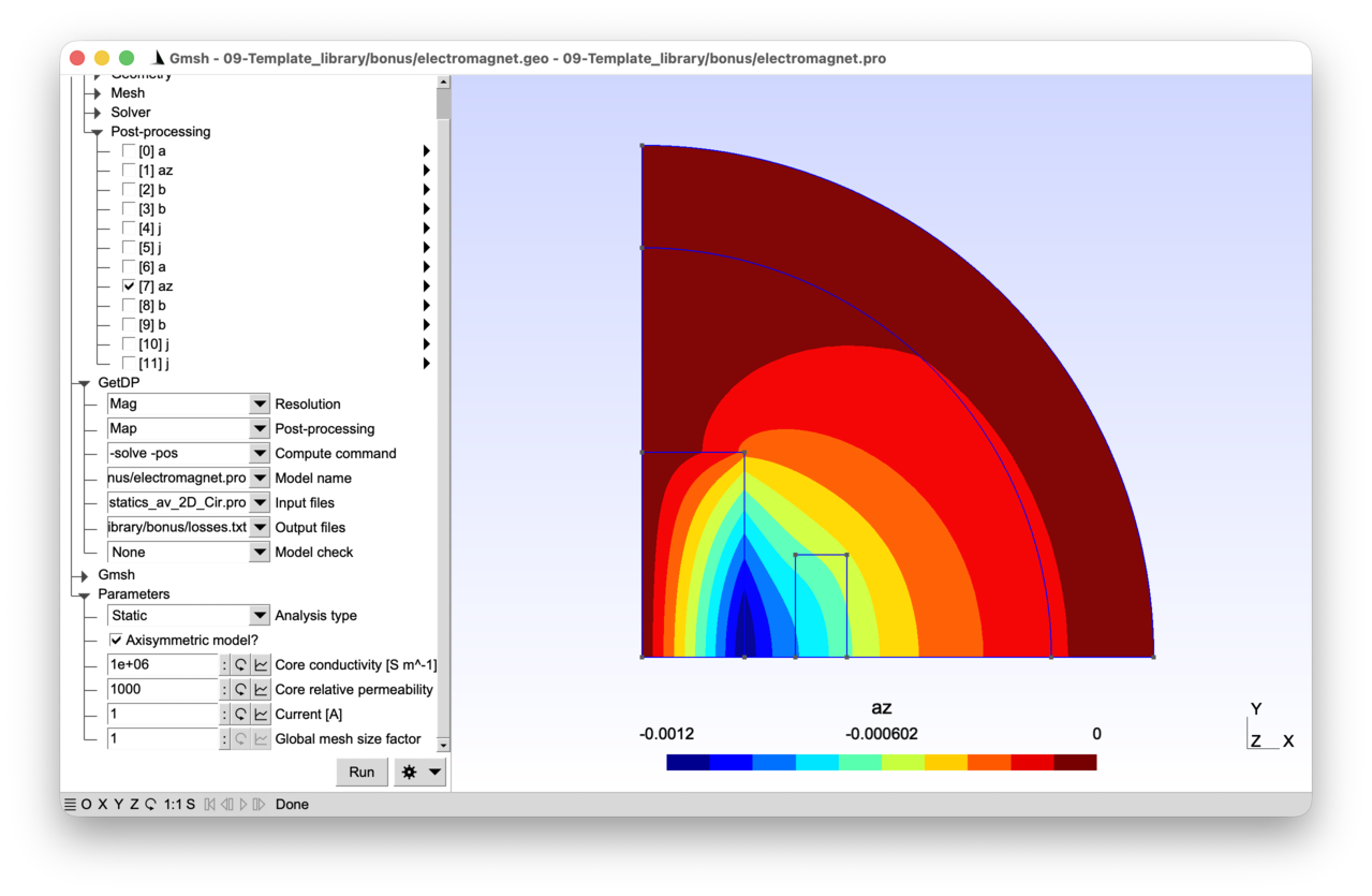
2.10.1 Running the tutorial 
On the command line:
> gmsh electromagnet.geo -2
> getdp electromagnet.pro -solve Mag -pos Map
Interactively with Gmsh: open electromagnet.pro with “File->Open”, then press “Run”.
2.10.2 Contents 
File electromagnet_common.pro 
// Parameters shared by Gmsh and GetDP.

mm = 1e-3;

dxCore = 50 * mm;
dyCore = 100 * mm;
xCoil = 75 * mm;
dxCoil = 25 * mm;
dyCoil = 100 * mm;
rInt = 200 * mm;
rExt = 250 * mm;
File electromagnet.geo 
// Gmsh script describing the geometry of the electromagnet. This is a pared
// down version of the geometry from tutorial 3, where all symmetries are
// taken advantage of.

Include "electromagnet_common.pro";

SetFactory("OpenCASCADE");
Rectangle(1) = {-dxCore, -dyCore, 0, 2 * dxCore, 2 * dyCore};
Rectangle(2) = {xCoil, -dyCoil / 2, 0, dxCoil, dyCoil};
Rectangle(3) = {-xCoil - dxCoil, -dyCoil / 2, 0, dxCoil, dyCoil};
Disk(4) = {0, 0, 0, rInt};
Disk(5) = {0, 0, 0, rExt};
d = 1.1 * rExt;
Rectangle(6) = {0, 0, 0, d, d};
BooleanIntersection{ Surface{6}; Delete; }{ Surface{1:5}; Delete; }

core() = Closest{0, 0, 0}{ Surface{:}; };
air() = Closest{dxCore + mm, 0, 0}{ Surface{:}; };
airinf() = Closest{rInt + mm, 0, 0}{ Surface{:}; };
indr() = Closest{xCoil + mm, 0, 0}{ Surface{:}; };
Physical Surface("Core", 1) = core(0);
Physical Surface("Air", 2) = air(0);
Physical Surface("AirInf", 3) = airinf(0);
Physical Surface("CoilRight", 4) = indr(0);

bot() = Curve In BoundingBox{-mm, -mm, -mm, d, mm, mm};
left() = Curve In BoundingBox{-mm, -mm, -mm, mm, d, mm};
inf() = CombinedBoundary{ Surface{:}; };
inf() -= {bot(), left()};
Physical Curve("Bottom", 10) = bot();
Physical Curve("Left", 11) = left();
Physical Curve("Inf", 12) = inf();

// Mesh size constraints:
DefineConstant[
  s = {1, Name "Parameters/}Global mesh size factor"}
];

MeshSize{:} = 12.5 * mm * s;
MeshSize{ PointsOf{ Surface{indr(0)}; } } = 5 * mm * s;
MeshSize{ PointsOf{ Surface{core(0)}; } } = 4 * mm * s;

// Refine to capture the skin depth:
skin() = Curve In BoundingBox{dxCore - mm, -mm, -mm, dxCore + mm, d, mm};
MeshSize{ PointsOf{ Curve{skin(0)}; } } = 0.5 * mm * s;
File electromagnet.pro 
// This file reimplements the electromagnet models from tutorials 3 and 4 using
// the "Lib_Magnetoquasistatics_av_2D_Cir.pro" template library. The library
// acts as a black box that hides the complexity of the formulation, function
// spaces, resolution and post-processing: the user only needs to define groups,
// material properties and constraints. The resulting model file is compact, yet
// supports static, time-domain and frequency-domain analyses, with or without
// axisymmetry.

Include "electromagnet_common.pro";

Group {
  // Physical regions:
  Core = Region[ 1 ];
  Air = Region[ 2 ];
  AirInf = Region[ 3 ];
  CoilRight = Region[ 4 ];
  Bottom = Region[ 10 ];
  Left = Region[ 11 ];
  Inf = Region[ 12 ];

  // Abstract regions expected by the library. The inductor is a stranded coil
  // ("Vol_S_Mag"), the core is a massive conductor with eddy currents
  // ("Vol_C_Mag"):
  Vol_Mag     = Region[ {Air, AirInf, Core, CoilRight} ];
  Vol_S_Mag   = Region[ CoilRight ];
  Vol_C_Mag   = Region[ Core ];
  Vol_Inf_Mag = Region[ AirInf ];
}

Function {
  DefineConstant[
    AnalysisType = {0, Choices{0="Static", 1="Time-domain", 2="Frequency-domain"},
      Name "Parameters/Analysis type"}
    Axisymmetric = {0, Choices{0, 1},
      Name "Parameters/Axisymmetric model?"}
    Current = {1, Min 0.01, Max 100, Step 0.1,
      Name "Parameters/Current [A]"}
    f = {5, Min 1, Max 1000, Step 1, Visible AnalysisType > 0,
      Name "Parameters/Frequency [Hz]"}
    mur = {1000, Min 1, Max 5000, Step 1,
      Name "Parameters/Core relative permeability"}
    sigma = {1e6, Min 1, Max 1e6, Step 100,
      Name "Parameters/Core conductivity [S m^-1]"}
  ];

  T = 1 / f;
  dt = T / 20;
  tmax = 2 * T;

  mu0 = 4.e-7 * Pi;
  nu0 = 1 / mu0;
  nu [ Region[{Air, AirInf, CoilRight}] ] = nu0;
  nu [ Core ]  = 1 / (mur * mu0);

  sigma[ Core ] = sigma;
  sigma[ CoilRight ] = sigma;

  If(AnalysisType > 0)
    time_fct[] = F_Sin_wt_p[]{2 * Pi * f, 0};
    SkinDepth = DefineNumber[ 1e3 * Sqrt[2 / (2 * Pi * f * mur * mu0 * sigma)],
      Name "Parameters/Skin depth [mm]", ReadOnly];
  Else
    time_fct[] = 1;
  EndIf

  // Stranded coil parameters: these four definitions are all the library needs
  // to handle the 1000-turn inductor with imposed current:
  Ns[ CoilRight ] = 1000;
  Sc[ CoilRight ] = dxCoil * dyCoil;
  CoefGeo[ CoilRight ] = (Axisymmetric ? 2 * Pi : 1) * (-1);
  CoefGeo[ Core ] = (Axisymmetric ? 2 * Pi : 1);
}

Constraint {
  { Name a_Mag_2D;
    Case {
      { Region Left; Value 0.; }
      { Region Inf; Value 0.; }
    }
  }
  { Name Voltage_Mag_2D;
    Case {
      // Zero voltage on the core
      { Region Core; Value 0; }
    }
  }
  { Name Current_Mag_2D;
    Case {
      // Imposed current in the inductor:
      { Region CoilRight; Value Current; TimeFunction time_fct[]; }
    }
  }
}

// Configure and include the library:
JacRadiusInt = rInt;
JacRadiusExt = rExt;
Freq = f;
TimeFinal = tmax;
DeltaTime = dt;
CoefPower = (AnalysisType == 2) ? 0.5 : 1;
Include "../Lib_Magnetoquasistatics_av_2D_Cir.pro";

PostOperation {
  { Name Map; NameOfPostProcessing Mag;
    Operation {
      Print[ a, OnElementsOf Vol_Mag, File "a.pos" ];
      Print[ az, OnElementsOf Vol_Mag, File "az.pos" ];
      Print[ b, OnElementsOf Vol_Mag, File "b.pos" ];
      Print[ b, OnLine{{mm, mm, 0}{rInt, mm, 0}}{50}, File "cutb.pos" ];
      Print[ j, OnElementsOf Vol_S_Mag, File "js.pos" ];
      Print[ j, OnElementsOf Vol_C_Mag, File "j.pos" ];
      Print[ JouleLosses[Vol_C_Mag], OnGlobal, Format Table, File "losses.txt" ];
    }
  }
}
2.11 Tutorial 10: Tree-cotree and Coulomb gauging 
We consider a 3D version of the single-phase transformer of tutorial 9. The primary winding is driven by a voltage source and the secondary winding feeds a selectable load (resistance, inductance or capacitance). In 3D, the curl-curl equation does not uniquely determine the magnetic vector potential “a”: gradient fields must be removed by imposing a gauge condition. Two strategies are presented and can be selected at runtime: tree-cotree gauging as in tutorial 8 (which constrains the degrees of freedom on a spanning tree of the mesh) and Coulomb gauging (which enforces “div a = 0” weakly via a scalar Lagrange multiplier). Both produce the same magnetic flux density “b = curl a”.
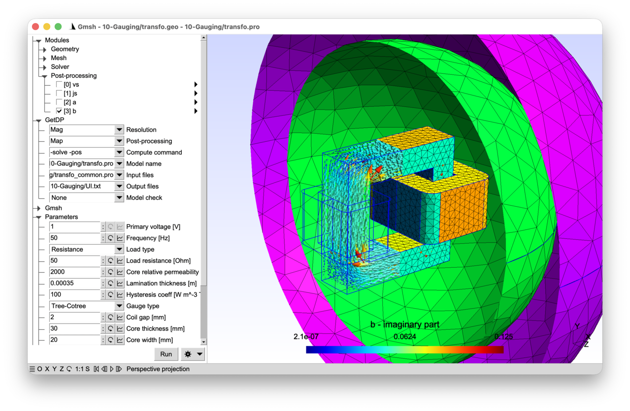
2.11.1 Features 
- 3D magneto-quasistatic formulation with circuit coupling
- Tree-cotree gauging via EdgesOfTreeIn / StartingOn
- Coulomb gauging via a mixed formulation with Lagrange multiplier
- Source current density obtained from an electrokinetic problem pre-computed on each coil
See the comments in transfo.pro and transfo.geo for details.
2.11.2 Running the tutorial 
On the command line:
> gmsh transfo.geo -3
> getdp transfo.pro -solve Mag -pos Map
Interactively with Gmsh: open transfo.pro with “File->Open”, then press “Run”.
2.11.3 Contents 
File transfo_common.pro 
// Parameters shared by Gmsh and GetDP: core and coil dimensions.

mm = 1e-3;
wCore = 100 * mm;
hCore = 100 * mm;
wCoil1 = 10 * mm;
hCoil1 = 40 * mm;
wCoil2 = 20 * mm;
hCoil2 = 40 * mm;

DefineConstant[
  thickCore = {30, Min 5, Max 60, Step 0.1,
    Name "Parameters/Core thickness [mm]"}
  gapCoil = {2, Min 0.5, Max 7.5, Step 0.1,
    Name "Parameters/Coil gap [mm]"}
  wCoreLeg = {20, Min 10, Max 27, Step 0.1,
    Name "Parameters/Core width [mm]"}
];

thickCore = thickCore * mm;
gapCoil = gapCoil * mm;
wCoreLeg = wCoreLeg * mm;

// Inner and outer radii for the infinite shell Jacobian (see tutorial 3),
// chosen to be large enough to enclose the full geometry:
r = Max[(wCore + 2 * gapCoil + wCoil1 + wCoil2) / 2, hCore / 2];
r = Max[r, (thickCore + 2 * gapCoil + Max[wCoil1, wCoil2]) / 2];
JacRadiusInt = r * Sqrt[2] + 30 * mm;
JacRadiusExt = JacRadiusInt + 50 * mm;
File transfo.geo 
// Gmsh script describing the geometry of the same single-phase transformer as
// in tutorial 9, but in 3D.

SetFactory("OpenCASCADE");

Include "transfo_common.pro";

// The core is created by subtracting the inner box (the window) from the
// outer box:
Box(1) = {-wCore / 2, -hCore / 2, -thickCore / 2,
  wCore, hCore, thickCore};
Box(2) = {-wCore / 2 + wCoreLeg, -hCore / 2 + wCoreLeg, -thickCore / 2,
  wCore - 2 * wCoreLeg, hCore - 2 * wCoreLeg, thickCore};
BooleanDifference(3) = { Volume{1}; Delete; }{ Volume{2}; Delete; };

// We define a macro to create a coil, which expects three input parameters to
// be defined:
//  - "xCoil": leftmost position of the coil
//  - "wCoil": width of the coil
//  - "hCoil": height of the coil
Macro Coil
  r1 = news; // "news" returns the next available surface tag
  Rectangle(r1) = {xCoil, -hCoil / 2,
    thickCore / 2 + gapCoil + wCoil,
    2 * wCoil + 2 * gapCoil + wCoreLeg,
    thickCore + 2 * gapCoil + 2 * wCoil,
    wCoil / 2}; // rounded corner with radius "wCoil / 2"
  r2 = news;
  Rectangle(r2) = {xCoil + wCoil, -hCoil / 2 + wCoil,
    thickCore / 2 + gapCoil + wCoil,
    wCoreLeg + 2 * gapCoil,
    thickCore + 2 * gapCoil};
  // Subtract the inner rectangle from the outer rounded rectangle:
  d() = BooleanDifference{ Surface{r1}; Delete; }{ Surface{r2}; Delete; };
  // Rotate the resulting surface to create the base of the coil:
  Rotate {{1, 0, 0}, {0, -hCoil / 2, thickCore / 2 + gapCoil + wCoil}, -Pi / 2} {
    Surface{d(0)};
  }
  // Extrude the base along the y-axis:
  e() = Extrude{0, hCoil, 0}{ Surface{d(0)}; };
  // Create a "cut" in the coil to define an electrode. The cut surface
  // is needed in 3D so that the source current density inside the coil
  // can be derived from a single-valued scalar potential, with a unit
  // jump across the cut (see the .pro file).
  r3 = news;
  Rectangle(r3) = {xCoil, -hCoil / 2, 0, wCoil, hCoil};
  BooleanFragments { Surface{r3}; Delete; }{ Volume{e(1)}; Delete; }
Return

// Call the "Coil" macro twice to create the two coils:
xCoil = -wCore / 2 - gapCoil - wCoil1;
wCoil = wCoil1;
hCoil = hCoil1;
Call Coil;
xCoil = wCore / 2 - wCoreLeg - gapCoil - wCoil2;
wCoil = wCoil2;
hCoil = hCoil2;
Call Coil;

// Create the spherical shell region:
Sphere(10) = {0, 0, 0, JacRadiusInt};
Sphere(11) = {0, 0, 0, JacRadiusExt};

// Fragment all entities to get a conformal geometry:
Coherence;

// Use the "Closest" command to retrieve the regions of interest:
coil1() = Closest {-wCore / 2 - gapCoil - wCoil1 / 2, 0, 0} { Volume{:}; };
elec1() = Closest {-wCore / 2 - gapCoil - wCoil1 / 2, 0, 0} { Surface{:}; };
coil2() = Closest {wCore / 2 + gapCoil + wCoil2 / 2, 0, 0} { Volume{:}; };
elec2() = Closest {wCore / 2 - wCoreLeg - gapCoil - wCoil2 / 2, 0, 0} { Surface{:}; };
core() = Closest {0, hCore / 2 - mm, 0} { Volume{:}; };
airinf() = Closest {JacRadiusInt + mm, 0, 0} { Volume{:}; };

air() = Volume{:};
air() -= {airinf(0), core(0), coil1(0), coil2(0)};
bnd() = CombinedBoundary{ Volume{:}; };

// Assign mesh sizes:
DefineConstant[
  s = {3, Min 0.1, Max 10, Step 0.1,
    Name "Parameters/}Global mesh size factor"}
];
MeshSize{:} = 2 * mm * s;
MeshSize{ PointsOf{ Volume{airinf(0)}; } } = 8 * mm * s;

// Create physical groups:
Physical Volume("Air", 1) = air();
Physical Volume("AirInf", 2) = airinf(0);
Physical Volume("Coil1", 3) = coil1(0);
Physical Volume("Coil2", 4) = coil2(0);
Physical Volume("Core", 5) = core(0);
Physical Surface("Bnd", 10) = bnd();
Physical Surface("Electrode1", 11) = elec1(0);
Physical Surface("Electrode2", 12) = elec2(0);
File transfo.pro 
// GetDP formulation for same transformer model as in tutorial 9, but in 3D. The
// 3D vector potential "a" requires gauging for uniqueness in 3D; this tutorial
// presents two strategies, selectable via the "GaugeType" parameter:
// tree-cotree gauging and Coulomb gauging (through a Lagrange multiplier).

// Resolution sequence: we first pre-compute a normalized source current density
// in each coil, then link it to global variables for field-circuit coupling in
// the 3D a-v formulation. The actual source current density is enforced in each
// coil by multiplying the pre-computed distribution by the global current
// quantity computed from the circuit equations.
Include "transfo_common.pro";

Group {
  // Physical regions:
  Air = Region[ 1 ];
  AirInf = Region[ 2 ];
  Coil_1 = Region[ 3 ];
  Coil_2 = Region[ 4 ];
  Coils = Region[ {Coil_1, Coil_2} ];
  Core = Region[ 5 ];
  Bnd = Region[ 10 ];
  Electrode_1 = Region[ 11 ];
  Electrode_2 = Region[ 12 ];

  // Abstract regions:
  //  - "Vol_Mag": full magnetic domain
  //  - "Vol_S_Mag": stranded conductors (windings with Ns turns)
  //  - "Vol_Inf_Mag": region with infinite shell transformation
  //  - "Vol_Ele~{i}": i-th coil for source current density pre-calculation
  //  - "Sur_Electrode_Ele~{i}": electrode in i-th coil
  Vol_Mag = Region[ {Air, AirInf, Core, Coil_1, Coil_2} ];
  Vol_S_Mag = Region[ {Coil_1, Coil_2} ];
  Vol_Inf_Mag = Region[ AirInf ];
  NumCoils = 2;
  For i In {1 : NumCoils}
    // "~{i}" in the group names below will be transformed into "_1" when "i ==
    // 1" and "_2" when "i == 2" in the "For" loop. This is a general mechanism
    // in GetDP that can be applied not only to groups but to most object names
    // (constants, functions, constraints, function spaces, ...) in order to
    // create their names programmatically:
    Vol_Ele~{i} = Region[ Coil~{i} ];
    Sur_Electrode_Ele~{i} = Region[ Electrode~{i} ];
  EndFor

  // Circuit regions:
  E_in = Region[ 100 ];
  Z_out = Region[ 102 ];

  // Abstract circuit regions:
  //  - "Source_Cir": all voltage and current sources
  //  - "Resistance_Cir": all resistors
  //  - "Inductance_Cir": all inductors
  //  - "Capacitance_Cir": all capacitors
  Source_Cir = Region[ {E_in} ];
  DefineConstant[
    LoadType = {0, Choices {0="Resistance", 1="Inductance", 2="Capacitance"},
      Name "Parameters/2Load type"}
  ];
  If(LoadType == 0)
    Resistance_Cir = Region[ {Z_out} ];
  ElseIf(LoadType == 1)
    Inductance_Cir = Region[ {Z_out} ];
  Else
    Capacitance_Cir = Region[ {Z_out} ];
  EndIf
}

Function {
  DefineConstant[
    Voltage = {1, Min 1e-3, Max 10,
      Name "Parameters/0Primary voltage [V]"}
    f = {50, Min 0, Max 1e3, Step 1,
      Name "Parameters/1Frequency [Hz]"}
    Rval = {50, Min 1e-3, Max 50, Step 0.25, Visible (LoadType == 0),
      Name "Parameters/3Load resistance [Ohm]"}
    Lval = {1e-6, Min 1e-9, Max 0.1, Step 1e-3, Visible (LoadType == 1),
      Name "Parameters/3Load inductance [H]"}
    Cval = {1e-6, Min 1e-9, Max 0.1, Step 1e-4, Visible (LoadType == 2),
      Name "Parameters/3Load capacitance [F]"}
    murCore = {2000, Min 1, Max 10000, Step 1,
      Name "Parameters/4Core relative permeability"}
    dlam = {0.35e-3, Min 0.1e-3, Max 1e-3, Step 0.05e-3,
      Name "Parameters/5Lamination thickness [m]"}
    kh = {100, Min 10, Max 500, Step 10,
      Name "Parameters/6Hysteresis coeff [W m^-3 T^-2 s]"}
    GaugeType = {0, Choices {0="Tree-Cotree", 1="Coulomb"},
      Name "Parameters/7Gauge type"}
  ];

  mu0 = 4e-7 * Pi;
  nu[ Air ] = 1 / mu0;
  nu[ AirInf ] = 1 / mu0;

  // Same modelling of ferromagnetic laminations as in tutorial 9:
  nu_r = 1 / (murCore * mu0);
  sigma_iron = 2e6;
  nu_i = kh / Pi + sigma_iron * (2 * Pi * f) * dlam^2 / 12;
  nu[ Core ] = Complex[nu_r, nu_i];

  // Number of turns "Ns" of each coil:
  Ns[ Coil_1 ] = 100;
  Ns[ Coil_2 ] = 200;

  nu[ Coils ] = 1 / mu0;
  sigma[ Coils ] = 5.8e7;

  Resistance[ Z_out ] = Rval;
  Inductance[ Z_out ] = Lval;
  Capacitance[ Z_out ] = Cval;
}

Constraint {
  { Name a_Mag;
    Case {
      { Region Bnd; Value 0; }
    }
  }

  // Tree-cotree gauging constraint on the vector potential "a" (only used when
  // "GaugeType == 0"); "a" is set to zero on the edges of a spanning tree of
  // the mesh; the "SubRegion Bnd" anchors the tree on the outer boundary, where
  // the homogeneous Dirichlet boundary condition "a_Mag" is imposed:
  { Name a_Gauge_Mag;
    Case {
      { Region Vol_Mag ; SubRegion Bnd; Value 0.; }
    }
  }

  // Boundary condition for the Coulomb gauge multiplier "xi" (only used when
  // "GaugeType == 1"):
  { Name xi_Mag;
    Case {
      // N.B.: we are only interested in the gradient of "xi", so we can set "xi"
      // to any value on the boundary; here we choose zero as it allows for an
      // easier mixed formulation (see explanations in the "Formulation" below):
      { Region Bnd; Value 0; }
    }
  }

  // No imposed current or voltage in the magnetic formulation -- the voltage
  // source is imposed in the circuit as in tutorial 9:
  { Name Current_Mag;
    Case {
    }
  }
  { Name Voltage_Mag;
    Case {
    }
  }

  { Name Current_Cir ;
    Case {
    }
  }

  { Name Voltage_Cir ;
    Case {
      { Region E_in; Value Voltage; TimeFunction F_Cos_wt_p[]{2 * Pi * f, 0}; }
    }
  }

  // Contrary to the massive conductor case (see tutorial 8), the global basis
  // function for circuit coupling is not associated with the electrodes
  // anymore, but directly with the regions in "Vol_S_Mag", i.e., with "Coil_1"
  // and "Coil_2", through the use of the pre-computed source current density
  // with "BF_Global" in the "Hregion_vs_Mag" function space (see below):
  { Name ElectricalCircuit ; Type Network ;
    Case Circuit_1 {
      { Region E_in; Branch {1, 2}; }
      { Region Coil_1; Branch {2, 1} ; }
    }
    Case Circuit_2 {
      { Region Coil_2; Branch {1, 2} ; }
      { Region Z_out; Branch {2, 1}; }
    }
  }
}

Jacobian {
  { Name Vol;
    Case {
      { Region All; Jacobian Vol; }
    }
  }
  { Name Sur;
    Case {
      { Region All; Jacobian Sur; }
    }
  }
}

Integration {
  { Name Int;
    Case {
      { Type Gauss;
        Case {
          { GeoElement Line; NumberOfPoints 4; }
          { GeoElement Triangle; NumberOfPoints 4; }
          { GeoElement Tetrahedron; NumberOfPoints 4; }
        }
      }
    }
  }
}

Group {
  DefineGroup[ Source_Cir, Resistance_Cir, Inductance_Cir, Capacitance_Cir ];
  Dom_Cir = Region[ {Source_Cir, Resistance_Cir, Inductance_Cir,
      Capacitance_Cir} ];
}

// Pre-computation of the source current density distribution in each coil. The
// scalar potential "vs" solves a homogeneous Laplace problem on the coil
// volume, with a unit jump across the electrode (the cut introduced in the
// .geo). The resulting field "js = -grad(vs)" is therefore divergence-free and,
// by construction, integrates to one across any cross-section. Below, each "js"
// field will be multiplied by the net current in Coil~{i} to model the actual
// current density distribution in the coil.
//
// Note that "js" is not exactly uniform across the cross-section: like a DC
// current in a homogeneous solid conductor of the same shape, it concentrates
// on the inner side of bends, where the current path is shorter. For a stranded
// winding (whose ideal current density would be uniform along the wire axis,
// "js = tau / Sc" with "tau" the unit tangent), this is therefore an
// approximation. Alternatives include prescribing "js" analytically (only
// practical for simple shapes like straight or circular coils), computing it
// from a magnetostatic problem with a known driving current (e.g. via
// Biot-Savart for line segments), or homogenizing the winding. The Laplace
// approach used here is fully general and divergence-free by construction.

For i In {1 : NumCoils}

  Constraint {
    // We enforce unit current across each coil's electrode
    { Name UnitCurrent~{i};
      Case {
        { Region Sur_Electrode_Ele~{i}; Type Assign; Value 1; }
      }
    }
  }

  FunctionSpace {
    { Name H1_vs~{i}; Type Form0;
      BasisFunction {
        { Name sn; NameOfCoef vn; Function BF_Node;
          Support Vol_Ele~{i};
          Entity NodesOf[ All, Not Sur_Electrode_Ele~{i} ]; }
        // We restrict the support of the global basis function to the positive
        // side of the electrode, i.e. the side where the electrode normal
        // points, using "ElementsOf[ ..., OnPositiveSideOf ...]". Since the
        // electrode surface "Sur_Electrode_Ele~{i}" is connected on both sides
        // to the same coil volume "Coil~{i}", this is necessary to properly set
        // up the discontinuity of "vs": the negative side of the electrode in
        // "Coil~{i}" will not be part of the support, hence the global function
        // will evaluate to zero there.
        //
        // As an alternative, we could have cut each "Coil~{i}" volume into two
        // parts, and restricted the support of the global function to one of
        // the parts.
        { Name sf; NameOfCoef vf; Function BF_GroupOfNodes;
          Support ElementsOf[Vol_Ele~{i}, OnPositiveSideOf Sur_Electrode_Ele~{i}];
          Entity GroupsOfNodesOf[ Sur_Electrode_Ele~{i} ]; }
      }
      GlobalQuantity {
        { Name Voltage; Type AliasOf; NameOfCoef vf; }
        { Name Current; Type AssociatedWith; NameOfCoef vf; }
      }
      Constraint {
        { NameOfCoef Current; EntityType GroupsOfNodesOf;
          NameOfConstraint UnitCurrent~{i}; }
      }
    }
  }

  Formulation {
    { Name Electrokinetics_vs~{i}; Type FemEquation;
      Quantity {
        { Name vs; Type Local; NameOfSpace H1_vs~{i}; }
        { Name I; Type Global; NameOfSpace H1_vs~{i} [Current]; }
        { Name V; Type Global; NameOfSpace H1_vs~{i} [Voltage]; }
      }
      Equation {
        Integral { [ Dof{d vs} , {d vs} ];
          In Vol_Ele~{i}; Jacobian Vol; Integration Int; }
        GlobalTerm { [ Dof{I} , {V} ]; In Sur_Electrode_Ele~{i}; }
      }
    }
  }

  Resolution {
    // The "Ele~{i}" resolutions will be triggered automatically in a
    // pre-resolution phase, due to the "BF_Global" definition below; we hide
    // these resolutions from the list of available resolutions with the "Hidden
    // 1" option:
    { Name Ele~{i}; Hidden 1;
      System {
        { Name Sys_Ele; NameOfFormulation Electrokinetics_vs~{i}; }
      }
      Operation {
        Generate[Sys_Ele]; Solve[Sys_Ele];
      }
    }
  }

EndFor

FunctionSpace {

  // Function space for the magnetic vector potential "a". In 3D, the curl-curl
  // operator has a non-trivial kernel: since "curl(grad(phi)) = 0", any "a +
  // grad(phi)" gives the same flux density "b = curl(a)" and the same curl-curl
  // energy, so "a" is indeterminate up to gradients of arbitrary scalars "phi
  // in H1_0". A gauge condition is needed to obtain a unique solution:
  //  - Tree-cotree gauging ("GaugeType == 0"): pin "ae" to zero on the edges of
  //    a spanning tree of the mesh, rooted on the outer boundary
  //    ("EntitySubType StartingOn"). The gradient null space is spanned exactly
  //    by the tree edges (modulo boundary), so this kills it without affecting
  //    the physical solution. This constraint is directly implemented in the
  //    "Hcurl_a_Mag" space.
  //  - Coulomb gauging (GaugeType == 1): the gauge is imposed weakly in the
  //    formulation (see explanations in the "Formulation" below), thanks to a
  //    Lagrange multiplier "xi" in the "H1_xi_Mag" space.

  { Name Hcurl_a_Mag; Type Form1;
    BasisFunction {
      { Name se; NameOfCoef ae; Function BF_Edge;
        Support Vol_Mag; Entity EdgesOf[All]; }
    }
    Constraint {
      { NameOfCoef ae; EntityType EdgesOf; NameOfConstraint a_Mag; }
      If (GaugeType == 0)
        { NameOfCoef ae; EntityType EdgesOfTreeIn; EntitySubType StartingOn;
          NameOfConstraint a_Gauge_Mag; }
      EndIf
    }
  }

  If (GaugeType == 1)
    // We introduce a scalar Lagrange multiplier "xi" in H1_0 to enforce the
    // Coulomb gauge constraint; see explanations in the "Formulation" below.
    { Name H1_xi_Mag ; Type Form0 ;
      BasisFunction {
        { Name sn ; NameOfCoef xin ; Function BF_Node ;
          Support Vol_Mag; Entity NodesOf[All]; }
      }
      Constraint {
        { NameOfCoef xin; EntityType NodesOf; NameOfConstraint xi_Mag; }
      }
    }
  EndIf

  // Function space for the stranded-conductor global DoFs: one current (and its
  // dual voltage) per coil. Each basis function is the entire spatial
  // distribution of "vs" pre-computed by "Electrokinetics_vs~{i}" on the
  // corresponding "Coil~{i}", and the associated coefficient "ir" is the actual
  // current flowing through that coil.
  { Name Hregion_vs_Mag; Type Form0;
    BasisFunction {
      { Name sr; NameOfCoef ir;
        // "BF_Global" builds a basis function from a quantity computed by
        // another formulation -- here the unit-current source distribution
        // "-grad(vs)" pre-computed for each coil. The number of global basis
        // functions ("NumCoils == 2") should coincide with the number of
        // regions in "Group Vol_S_Mag" ("Coil_1" and "Coil_2"). The special
        // syntax "Electrokinetics_vs {NumCoils}" for the "Formulation" expands
        // to "Electrokinetics_vs_1" and "Electrokinetics_vs_2", matched
        // one-to-one with the regions of "Group Vol_S_Mag". "Ele {NumCoils}"
        // expands in the same way to "Ele_1" and "Ele_2" for the "Resolution":
        Function BF_Global {
          Quantity vs; Formulation Electrokinetics_vs {NumCoils};
          Group Vol_S_Mag; Resolution Ele {NumCoils};
        };
        // Each global basis function is directly associated with a "Global"
        // entity, i.e. each region in "Vol_S_Mag":
        Support Vol_S_Mag; Entity Global [Vol_S_Mag]; }
    }
    // "Current" is an alias of the coefficient "ir" (so "Current" is directly
    // the coil's current). "Voltage" is the dual global quantity associated
    // with "ir", representing the coil's terminal voltage; the link between
    // them is established by the "GlobalTerm" in the formulation and closed by
    // the "Network" constraint.
    GlobalQuantity {
      { Name Current; Type AliasOf; NameOfCoef ir; }
      { Name Voltage; Type AssociatedWith; NameOfCoef ir; }
    }
    // Both globals are left free here (cf. the empty "Current_Mag" and
    // "Voltage_Mag" constraints above): their runtime values are set by the
    // circuit equations.
    Constraint {
      { NameOfCoef Current; EntityType Global; NameOfConstraint Current_Mag; }
      { NameOfCoef Voltage; EntityType Global; NameOfConstraint Voltage_Mag; }
    }
  }

  { Name Hregion_i_Cir; Type Scalar;
    BasisFunction {
      { Name sr; NameOfCoef ir; Function BF_Region;
        Support Dom_Cir; Entity Dom_Cir; }
    }
    GlobalQuantity {
      { Name Current; Type AliasOf; NameOfCoef ir; }
      { Name Voltage; Type AssociatedWith; NameOfCoef ir; }
    }
    Constraint {
      { NameOfCoef Voltage; EntityType Region; NameOfConstraint Voltage_Cir; }
      { NameOfCoef Current; EntityType Region; NameOfConstraint Current_Cir; }
    }
  }

}

Formulation {
  { Name Magnetoquasistatics_av; Type FemEquation;
    Quantity {
      { Name a; Type Local; NameOfSpace Hcurl_a_Mag; }
      If(GaugeType == 1)
        { Name xi ; Type Local ; NameOfSpace H1_xi_Mag; }
      EndIf

      { Name vs; Type Local ; NameOfSpace Hregion_vs_Mag; }
      { Name Is; Type Global; NameOfSpace Hregion_vs_Mag [Current]; }
      { Name Us; Type Global; NameOfSpace Hregion_vs_Mag [Voltage]; }

      { Name Iz; Type Global; NameOfSpace Hregion_i_Cir [Current]; }
      { Name Uz; Type Global; NameOfSpace Hregion_i_Cir [Voltage]; }
    }
    Equation {
      Integral { [ nu[] * Dof{d a} , {d a} ];
        In Vol_Mag; Jacobian Vol; Integration Int; }

      // The Coulomb gauge weakly imposes div(a) = 0 via a Lagrange multiplier
      // saddle-point formulation. It picks, within each equivalence class "a +
      // grad(H1_0)", the unique representative L^2-orthogonal to the kernel:
      //
      //   (a, grad(xi')) = 0,   for all xi' in H1_0                 (*)
      //
      // By integration by parts ("xi' = 0" on "Bnd" cancels the boundary term),
      // (*) is equivalent to the variational form of "div(a) = 0", hence the
      // name.
      //
      // The constraint (*) is enforced by introducing a Lagrange multiplier "xi
      // in H1_0" and forming the Lagrangian
      //
      //   L(a, xi) = (1/2) * (nu * curl(a), curl(a)) - (j, a) + (a, grad(xi)).
      //
      // The two stationarity conditions give the saddle-point system. Variation
      // in "a" (replace "a" by "a + eps * a'", differentiate "L" with respect
      // to "eps" and set to zero at "eps = 0") gives, for any test direction
      // "a'", the augmented curl-curl equation
      //
      //   (nu * curl(a), curl(a')) + (grad(xi), a') = (j, a')       (1)
      //
      // The same procedure for "xi" affects only the multiplier-coupling term
      // and gives the gauge constraint
      //
      //   (a, grad(xi')) = 0                                        (2)
      //
      // (The term "(grad(xi), a')" in (1) is the transpose of "(a, grad(xi'))"
      // in (2), making the off-diagonal blocks of the block system transposes
      // of each other and the system symmetric.)
      //
      // Note: an "augmented Lagrangian" variant adds a penalty term "(gamma /
      // 2) * (div(a), div(a))" to "L", contributing an extra "gamma * (div(a),
      // div(a'))" to equation (1). With "gamma > 0" this improves the
      // conditioning of the otherwise indefinite system at the cost of tuning
      // "gamma"; the implementation below uses the bare Lagrangian ("gamma ==
      // 0"):
      If(GaugeType == 1)
        Integral { [ Dof{a}, {d xi} ] ;
          In Vol_Mag; Jacobian Vol; Integration Int; }
        Integral { [ Dof{d xi}, {a} ] ;
          In Vol_Mag; Jacobian Vol; Integration Int; }
      EndIf

      // The pre-computed source distribution "-grad(vs)" is normalized to a
      // unit current across the cross-section; the "Ns" factor scales it up to
      // the actual current density of the Ns-turn winding. The minus sign on
      // the dual term reflects "j_unit = -grad(vs)": the flux linkage "Lambda =
      // Ns * (a, j_unit) = -Ns * (a, grad(vs))" and its time derivative (the
      // back-EMF in the voltage equation) thus carry the opposite sign of the
      // source term:
      Integral { [ Ns[] * Dof{d vs} , {a} ];
        In Vol_S_Mag; Jacobian Vol; Integration Int; }

      Integral { DtDof[ -Ns[] * Dof{a} , {d vs} ];
        In Vol_S_Mag; Jacobian Vol; Integration Int; }

      // DC resistance of the winding. The "Ns^2" factor comes from Ns turns in
      // series, each one with cross-section Sc/Ns and length proportional to
      // Ns, i.e. R_total = Ns^2 * L / (sigma * Sc):
      Integral { [ Ns[]^2 / sigma[] * Dof{d vs} , {d vs} ];
        In Vol_S_Mag; Jacobian Vol; Integration Int; }

      GlobalTerm { [ Dof{Us} , {Is} ]; In Vol_S_Mag; }

      // The circuit coupling is handled in the same way as in tutorials 8 and
      // 9:
      GlobalTerm { [ Dof{Uz} , {Iz} ]; In Resistance_Cir; }
      GlobalTerm { [ Resistance[] * Dof{Iz} , {Iz} ]; In Resistance_Cir; }

      GlobalTerm { [ Dof{Uz} , {Iz} ]; In Inductance_Cir; }
      GlobalTerm { DtDof [ Inductance[] * Dof{Iz} , {Iz} ]; In Inductance_Cir; }

      GlobalTerm { [ Dof{Iz} , {Iz} ]; In Capacitance_Cir; }
      GlobalTerm { DtDof [ Capacitance[] * Dof{Uz} , {Iz} ]; In Capacitance_Cir; }

      GlobalEquation {
        Type Network; NameOfConstraint ElectricalCircuit;
        { Node {Is}; Loop {Us}; Equation {Us}; In Vol_S_Mag; }
        { Node {Iz}; Loop {Uz}; Equation {Uz}; In Dom_Cir; }
      }
    }
  }
}

Resolution {
  { Name Mag;
    System {
      { Name Sys_Mag; NameOfFormulation Magnetoquasistatics_av;
        Type Complex; Frequency f;
      }
    }
    Operation {
      Generate[Sys_Mag]; Solve[Sys_Mag]; SaveSolution[Sys_Mag];
    }
  }
}

PostProcessing {
  { Name Mag; NameOfFormulation Magnetoquasistatics_av;
    Quantity {
      { Name a;
        Value {
          Term { [ {a} ]; In Vol_Mag; Jacobian Vol; }
        }
      }
      { Name vs;
        Value {
          Term { [ {vs} ]; In Vol_S_Mag; Jacobian Vol; }
        }
      }
      { Name js;
        Value {
          Term { [ - {d vs} ]; In Vol_S_Mag; Jacobian Vol; }
        }
      }
      { Name b;
        Value {
          Term { [ {d a} ]; In Vol_Mag; Jacobian Vol; }
        }
      }
      { Name U; Value {
          Term { [ {Uz} ]; In Dom_Cir; }
          Term { [ {Us} ]; In Vol_S_Mag; }
        }
      }
      { Name I; Value {
          Term { [ {Iz} ]; In Dom_Cir; }
          Term { [ {Is} ]; In Vol_S_Mag; }
        }
      }
      { Name NormU; Value {
          Term { [ Norm[{Uz}] ]; In Dom_Cir; }
          Term { [ Norm[{Us}] ]; In Vol_S_Mag; }
        }
      }
      { Name NormI; Value {
          Term { [ Norm[{Iz}] ]; In Dom_Cir; }
          Term { [ Norm[{Is}] ]; In Vol_S_Mag; }
        }
      }
    }
  }
}


PostOperation {
  { Name Map; NameOfPostProcessing Mag;
    Operation {
      Print[ vs, OnElementsOf Vol_S_Mag, Format Gmsh, File "vs.pos" ];
      Print[ js, OnElementsOf Vol_S_Mag, Format Gmsh, File "js.pos" ];
      Print[ a, OnElementsOf Vol_Mag, Format Gmsh, File "a.pos" ];
      Print[ b, OnElementsOf Vol_Mag, Format Gmsh, File "b.pos" ];
      Echo[ "E_in", Format Table, File "UI.txt" ];
      Print[ U, OnRegion E_in, Format FrequencyTable, File > "UI.txt"];
      Print[ I, OnRegion E_in, Format FrequencyTable, File > "UI.txt"];
      Echo[ "Z_out", Format Table, File > "UI.txt" ];
      Print[ U, OnRegion Z_out, Format FrequencyTable, File > "UI.txt"];
      Print[ I, OnRegion Z_out, Format FrequencyTable, File > "UI.txt"];
      Print[ NormU, OnRegion E_in, Format Table, File "",
        SendToServer "}Output/0|V_in| [V]"{0} ];
      Print[ NormI, OnRegion E_in, Format Table, File "",
        SendToServer "}Output/1|I_in| [A]"{0} ];
      Print[ NormU, OnRegion Z_out, Format Table, File "",
        SendToServer "}Output/2|V_out| [V]"{0} ];
      Print[ NormI, OnRegion Z_out, Format Table, File "",
        SendToServer "}Output/3|I_out| [A]"{0} ];
    }
  }
}
3 GetDP command-line interface 
On the command line, GetDP takes as arguments a single input file name followed by options:
> getdp filename options
where filename is the ASCII .pro file containing the problem definition. This file can include other files (see Comments and includes), so that only a single .pro file should always be given on the command line. The base name of this file (without the .pro extension) is used as a basis for the creation of intermediate files during the pre-processing, resolution and processing stages.
The options are a combination of the following commands (in any order):
-pre¶resolution-id
Performs the pre-processing associated with the resolution resolution-id. In the pre-processing stage, GetDP creates the geometric database (from the mesh file), identifies the degrees of freedom (the unknowns) of the problem and sets up the constraints on these degrees of freedom. The pre-processing creates a file with a .pre extension. If resolution-id is omitted, the list of available choices is displayed.
-cal¶-
Performs the processing. This requires that a pre-processing has been performed previously, or that a
-preoption is given on the same command line. The performed resolution is the one given as an argument to the-preoption. In the processing stage, GetDP executes all the commands given in theOperationfield of the selectedResolutionobject (such as matrix assemblies, system resolutions, …). -pos¶post-operation-id …
Performs the operations in the
PostOperation(s) selected by the post-operation-id(s). This requires that a processing has been performed previously, or that a-caloption is given on the same command line. If post-operation-id is omitted, the list of available choices is displayed.-msh¶filename
Reads the mesh (in
.mshformat) from filename rather than from the default problem file name (with the .msh extension appended).-msh_scaling¶value
Multiplies the coordinates of all the nodes in the mesh by value.
-gmshread¶filename …
Read gmsh data files (same as GmshRead in
Resolutionoperations). Allows to use such datasets outside resolutions (e.g. in pre-processing).-split¶-
Saves processing results in separate files (one for each timestep).
-res¶filename …
Loads processing results from file(s).
-name¶string
Uses string as the default generic file name for input or output of mesh, pre-processing and processing files.
-restart¶-
Restarts processing of a time stepping resolution interrupted before being complete.
-solve¶resolution-id
Same as
-pre resolution-id -cal.-solver¶filename
Specifies a solver option file (whose format varies depending on the linear algebra toolkit used).
-slepc¶-
Uses SLEPc instead of Arpack as eigensolver.
-adapt¶file
Reads adaptation constraints from file.
-order¶real
Specifies the maximum interpolation order.
-cache¶-
Caches lump element circuit computations to disk.
-sparsity¶-
Computes the sparsity and parallel matrix layout once per system.
-sparsity-all¶-
Always computes sparsity and parallel matrix layout.
-bin¶-
Selects binary format for output files.
-v2¶-
Creates mesh-based Gmsh output files when possible.
-check¶-
Lets you check the problem structure interactively.
-v¶-verbose¶integer
Sets the verbosity level. A value of 0 means that no information will be displayed during the processing.
-cpu¶-
Reports CPU times for all operations.
-p¶-progress¶integer
Sets the progress update rate. This controls the refreshment rate of the counter indicating the progress of the current computation (in %).
-onelab¶name <address>
Communicates with OneLab (file or server address)
-setnumber¶name value
Sets constant number name to value
-setstring¶name value
Sets constant string name to value
-info¶-
Displays the version information.
-version¶-
Displays the version number.
-help¶-
Displays a message listing basic usage and available options.
4 GetDP problem definition language 
Here are the rules used to describe the GetDP problem definition syntax:
- Keywords and literal symbols are printed like
this. - Metasyntactic variables (i.e., text bits that are not part of the syntax, but stand for other text bits) are printed like this.
- A colon (
:) after a metasyntactic variable separates the variable from its definition. - Optional rules are enclosed in
<>pairs. - Multiple choices are separated by
|. - Three dots (…) indicate a possible repetition of the preceding rule.
- For conciseness, the notation
rule <, rule > …is replaced byrule <,…>. - The etc symbol replaces nonlisted rules.
An syntax index is provided at the end of this reference manual (see Syntax index).
- Expressions
Group: defining topological entitiesFunction: defining global and piecewise expressionsConstraint: specifying constraints on function spaces and formulationsFunctionSpace: building function spacesJacobian: defining jacobian methodsIntegration: defining integration methodsFormulation: building equationsResolution: solving systems of equationsPostProcessing: exploiting computational resultsPostOperation: exporting results- Comments and includes
- Macros, loops and conditionals
4.1 Expressions 
Expressions are the basic tool of GetDP. They cover a wide range of functional expressions, from constants to formal expressions containing functions (built-in or user-defined, depending on space and time, etc.), arguments, discrete quantities and their associated differential operators, etc. Note that ‘white space’ (spaces, tabs, new line characters) is ignored inside expressions (as well as inside all GetDP objects).
Expressions are denoted by the metasyntactic variable expression:
expression:
  ( expression ) |
  integer |
  real |
  constant-id |
  quantity |
  argument |
  current-value |
  variable-set |
  variable-get |
  register-set |
  register-get |
  operator-unary expression |
  expression operator-binary expression |
  expression operator-ternary-left expression operator-ternary-right expression |
  built-in-function-id [ < expression-list > ] < { expression-cst-list } > |
  function-id [ < expression-list > ] |
  < Real | Complex > [ expression ] |
  Dt [ expression ] |
  AtAnteriorTimeStep [ expression, integer ] |
  Order [ quantity ] |
  Trace [ expression, group-id ] |
  expression ##integer
The following sections introduce the quantities that can appear in expressions, i.e., constants (integer, real) and constant expression identifiers (constant-id, expression-cst-list), discretized field quantities (quantity), arguments (argument), current values (current-value), register values (register-set, register-get), operators (operator-unary, operator-binary, operator-ternary-left, operator-ternary-right) and built-in or user-defined functions (built-in-function-id, function-id). The last seven cases in this definition permit to cast an expression as real or complex, get the time derivative or evaluate an expression at an anterior time step, retrieve the interpolation order of a discretized quantity, evaluate the trace of an expression, and print the value of an expression for debugging purposes.
List of expressions are defined as:
expression-list:
  expression <,...>
4.1.1 Constants 
The three constant types used in GetDP are integer, real and string. These types have the same meaning and syntax as in the C or C++ programming languages. Besides general expressions (expression), purely constant expressions, denoted by the metasyntactic variable expression-cst, are also used:
expression-cst:
  ( expression-cst ) |
  integer |
  real |
  constant-id |
  operator-unary expression-cst |
  expression-cst operator-binary expression-cst |
  expression-cst operator-ternary-left expression-cst operator-ternary-right
      expression-cst |
  math-function-id [ < expression-cst-list > ] |
  #constant-id() |
  constant-id(expression-cst) |
  StrFind[ expression-char, expression-char ] |
  StrCmp[ expression-char, expression-char ] |
  StrLen[ expression-char ] |
  StringToName[ expression-char ] | S2N[ expression-char ] |
  Exists[ string ] | FileExists[ string ] | GroupExists[ string ] |
  GetForced[ string ] | NbrRegions [ string ] |
  GetNumber[ expression-char <, expression-cst> ]
StrFind searches the first expression-char for any
occurrence of the second expression-char. StrCmp compares
the two strings (returns an integer greater than, equal to, or less than
0, according as the first string is greater than, equal to, or less than
the second string). StrLen returns the length of the
string. StringToName creates a name from the provided
string. Exists checks for the existence of a constant or a
function. FileExists checks for the existence of a
file. GroupExists checks for the existence of a
group. GetForced gets the value of a constant (zero if does not
exist). NbrRegions counts the numbers of elementary regions in a
group. GetNumber allows to get the value of a ONELAB number
variable (the optional second argument specifies the default value
returned if the variable does not exist).
List of constant expressions are defined as:
expression-cst-list:
  expression-cst-list-item <,...>
with
expression-cst-list-item:
  expression-cst |
  expression-cst : expression-cst |
  expression-cst : expression-cst : expression-cst |
  constant-id () |
  constant-id ( { expression-cst-list } ) |
  List[ constant-id ] |
  List[ expression-cst-list-item ] |
  List[ { expression-cst-list } ] |
  ListAlt[ constant-id, constant-id ] |
  ListAlt[ expression-cst-list-item, expression-cst-list-item ] |
  LinSpace[ expression-cst, expression-cst, expression-cst ] |
  LogSpace[ expression-cst, expression-cst, expression-cst ] |
  - expression-cst-list-item |
  expression-cst * expression-cst-list-item |
  expression-cst-list-item * expression-cst |
  expression-cst / expression-cst-list-item |
  expression-cst-list-item / expression-cst |
  expression-cst-list-item ^ expression-cst |
  expression-cst-list-item + expression-cst-list-item |
  expression-cst-list-item - expression-cst-list-item |
  expression-cst-list-item * expression-cst-list-item |
  expression-cst-list-item / expression-cst-list-item |
  ListFromFile [ expression-char ] |
  ListFromServer [ expression-char ] |
  ReadTable [ expression-char, expression-char ]
The second case in this last definition permits to create a list
containing the range of numbers comprised between the two
expression-cst, with a unit incrementation step. The third case
also permits to create a list containing the range of numbers comprised
between the two expression-cst, but with a positive or negative
incrementation step equal to the third expression-cst. The fourth
and fifth cases permit to reference constant identifiers
(constant-ids) of lists of constants and constant identifiers of
sublists of constants (see below for the definition of constant
identifiers) . The sixth case is a synonym for the fourth. The seventh
case permits to create alternate lists: the arguments of ListAlt
must be constant-ids of lists of constants of the same
dimension. The result is an alternate list of these constants: first
constant of argument 1, first constant of argument 2, second constant of
argument 1, etc. These kinds of lists of constants are for example often
used for function parameters (see Functions). The next two cases
permit to create linear and logarithmic lists of numbers,
respectively. The remaining cases permit to apply arithmetic operators
item-wise in lists. ListFromFile reads a list of numbers from a
file. ListFromServer attemps to get a list of numbers from the
ONELAB variable expression-char. ReadTable reads tabular
data in the same format as ListFromFile, and in addition stores
in the run-time table named after the second expression-char.
Contrary to a general expression which is evaluated at runtime (thanks to an internal stack mechanism), an expression-cst is completely evaluated during the syntactic analysis of the problem (when GetDP reads the .pro file). The definition of such constants or lists of constants with identifiers can be made outside or inside any GetDP object. The syntax for the definition of constants is:
affectation:
  DefineConstant [ constant-id < = expression-cst > <,...> ]; |
  DefineConstant [ constant-id = { expression-cst , onelab-options } <,...> ]; |
  DefineConstant [ string-id < = string-def >  <,...> ]; |
  DefineConstant [ string-id = { string-def , onelab-options } <,...> ]; |
  constant-id <()> = constant-def; |
  constant-id = DefineNumber[ constant-def, onelab-options ];
  string-id <()> = string-def; |
  string-id = DefineString[ string-def, onelab-options ]; |
  Printf [ "string" ] < > | >> string-def >; |
  Printf [ "string", expression-cst-list ] < > | >> string-def >; |
  Read [ constant-id ] ; |
  Read [ constant-id , expression-cst ]; |
  UndefineConstant | Delete [ constant-id ] ;
  UndefineFunction [ constant-id ] ;
  SetNumber[ string , expression-cst ];
  SetString[ string , string-def ];
with
constant-id:
  string |
  string ( expression-cst-list ) |
  string ~ { expression-cst } <,...>

constant-def:
  expression-cst-list-item |
  { expression-cst-list }

string-id:
  string |
  string ~ { expression-cst } <,...>

string-def:
  "string" |
  StrCat[ expression-char <,...> ] |
  Str[ expression-char <,...> ]
Notes:
- Five constants are predefined in GetDP:
Pi(3.1415926535897932),0D(0),1D(1),2D(2) and3D(3). - When
~{expression-cst}is appended to a string string, the result is a new string formed by the concatenation of string,_(an underscore) and the value of the expression-cst. This is most useful in loops (see Macros, loops and conditionals), where it permits to define unique strings automatically. For example,For i In {1:3} x~{i} = i; EndForis the same as
x_1 = 1;
x_2 = 2;
x_3 = 3;
- The assignment in
DefineConstant(zero if no expression-cst is given) is performed only if constant-id has not yet been defined. This kind of explicit default definition mechanism is most useful in general problem definition structures making use of a large number of generic constants, functions or groups. When exploiting only a part of a complex problem definition structure, the default definition mechanism allows to define the quantities of interest only, the others being assigned a default value (that will not be used during the processing but that avoids the error messages produced when references to undefined quantities are made).When onelab-options are provided, the parameter is exchanged with the ONELAB server. See https://gitlab.onelab.info/doc/tutorials/wikis/ONELAB-syntax-for-Gmsh-and-GetDP for more information.
-
DefineNumberandDefineStringallow to define a ONELAB parameter. In this case the affectation always takes place.SetNumberandSetStringallow the direct setting of ONELAB parameters without defining local variables.
Character expressions are defined as follows:
expression-char:
  "string" |
  string-id |
  StrCat[ expression-char <,...> ] |
  Str[ expression-char <,...> ]
  StrChoice[ expression, expression-char, expression-char ] |
  StrSub[ expression-char, expression, expression ] |
  StrSub[ expression-char, expression ] |
  UpperCase [ expression-char ] |
  Sprintf [ expression-char ] |
  Sprintf[ expression-char, expression-cst-list ] |
  NameToString ( string ) | N2S ( string ) |
  GetString[ expression-char <, expression-char,> ] |
  Date | CurrentDirectory | CurrentDir |
  AbsolutePath [ expression-char ] |
  DirName [ expression-char ] |
  OnelabAction
StrCat and Str permit to concatenate
character expressions (Str adds a newline character after each
string except the last) when creating a string. Str is also used
to create string lists (when string-id is followed by
()). StrChoice returns the first or second
expression-char depending on the value of expression.
StrSub returns the portion of the string that starts at the
character position given by the first expression and spans the
number of characters given by the second expression or until the
end of the string (whichever comes first; or always if the second
expression is not provided). UpperCase converts the
expression-char to upper case. Sprintf is equivalent to the
sprintf C function (where expression-char is a format
string that can contain floating point formatting characters: %e,
%g, etc.). NameToString converts a variable name into a
string. GetString allows to get the value of a ONELAB string
variable (the optional second argument specifies the default value
returned if the variable does not exist.) Date permits to access
the current date. CurrentDirectory and CurrentDir return
the directory of the .pro file. AbsolutePath returns the
absolute path of a file. DirName returns the directory of a
file. OnelabAction returns the current ONELAB action
(e.g. check or compute).
List of character expressions are defined as:
expression-char-list:
  expression-char <,...>
4.1.2 Operators 
The operators in GetDP are similar to the corresponding operators in the C or C++ programming languages.
operator-unary:
-Unary minus.
!Logical not.
operator-binary:
^Exponentiation. The evaluation of the both arguments must result in a scalar value.
*Multiplication or scalar product, depending on the type of the arguments.
/\Cross product. The evaluation of both arguments must result in vectors.
/Division.
%Modulo. The evaluation of the second argument must result in a scalar value.
+Addition.
-Subtraction.
==Equality.
!=Inequality.
>Greater. The evaluation of both arguments must result in scalar values.
>=Greater or equality. The evaluation of both arguments must result in scalar values.
<Less. The evaluation of both arguments must result in scalar values.
<=Less or equality. The evaluation of both arguments must result in scalar values.
&&Logical ‘and’. The evaluation of both arguments must result in scalar values.
||Logical ‘or’. The evaluation of both arguments must result in floating point values. Warning: the logical ‘or’ always (unlike in C or C++) implies the evaluation of both arguments. That is, the second operand of
||is evaluated even if the first one is true.&Binary ‘and’.
|Binary ‘or’.
>>Bitwise right-shift operator. Shifts the bits of the first argument to the right by the number of bits specified by the second argument.
<<Bitwise left-shift operator. Shifts the bits of the first argument to the left by the number of bits specified by the second argument.
operator-ternary-left:
?
operator-ternary-right:
:The only ternary operator, formed by operator-ternary-left and operator-ternary-right is defined as in the C or C++ programming languages. The ternary operator first evaluates its first argument (the expression-cst located before the
?), which must result in a scalar value. If it is true (non-zero) the second argument (located between?and:) is evaluated and returned; otherwise the third argument (located after:) is evaluated and returned.
The evaluation priorities are summarized below (from stronger to weaker,
i.e., ^ has the highest evaluation priority). Parentheses
() may be used anywhere to change the order of evaluation.
^- (unary), !| &/\*, /, %+, -<, >, <=, >=, <<, >>!=, ==&&, ||?:
4.1.3 Functions 
Two types of functions coexist in GetDP: user-defined functions
(function-id, see Function: defining global and piecewise expressions) and built-in functions
(built-in-function-id, defined in this section).
Both types of functions are always followed by a pair of brackets
[] that can possibly contain arguments (see Arguments). This
makes it simple to distinguish a function-id or a
built-in-function-id from a constant-id. As shown below,
built-in functions might also have parameters, given between braces
{}, and which are completely evaluated during the analysis of
the syntax (since they are of expression-cst-list type):
built-in-function-id [ < expression-list > ] < { expression-cst-list } >
with
built-in-function-id:
  math-function-id |
  extended-math-function-id |
  green-function-id |
  geometry-function-id |
  physics-function-id |
  system-function-id
Notes:
- Classical mathematical functions (see Math functions) are the only functions allowed in a constant definition (see the definition of expression-cst in Constants).
4.1.4 Current values 
Current values return the current floating point value of an internal GetDP variable:
$TimeValue of the current time. This value is set to zero for non time dependent analyses.
$DTimeValue of the current time increment used in a time stepping algorithm.
$ThetaCurrent theta value in a theta time stepping algorithm.
$TimeStepNumber of the current time step in a time stepping algorithm.
$BreakpointIn case of a breakpoint hit in TimeLoopAdaptive it is the number of the current breakpoint. In the other case when $Time corresponds not to a breakpoint the value is -1.
$Iteration, $NLIterationCurrent iteration in a nonlinear loop.
$Residual, $NLResidualCurrent residual in a nonlinear loop.
$EigenvalueRealReal part of the current eigenvalue.
$EigenvalueImagImaginary part of the current eigenvalue.
$X, $XSValue of the current (destination or source) X-coordinate.
$Y, $YSValue of the current (destination or source) Y-coordinate.
$Z, $ZSValue of the current (destination or source) Z-coordinate.
$A, $B, $CValue of the current parametric coordinates used in the parametric
OnGridPostOperation.$QuadraturePointIndexIndex of the current quadrature point.
$KSPIterationCurrent iteration in a Krylov subspace solver.
$KSPResidualCurrent residual in a Krylov subspace solver.
$KSPIterationsTotal number of iterations of Krylov subspace solver.
$KSPConvergedReasonConvergence status of Krylov subspace solver (negative values indicate divergence; see PETSc
KSPConvergedReason).$KSPSystemSizeSystem size of Krylov subspace solver.
Note:
- The current X, Y and Z coordinates refer to the ‘physical world’ coordinates, i.e., coordinates in which the mesh is expressed.
Current values are “read-only”. User-defined run-time variables, which share the same syntax but whose value can be changed in an expression, are defined in Run-time variables and registers.
4.1.5 Arguments 
Function arguments can be used in expressions and have the following syntax (integer indicates the position of the argument in the expression-list of the function, starting from 1):
argument:
  $integer
4.1.6 Run-time variables and registers 
Constant expressions (expression-csts) are evaluated only once
during the analysis of the problem definition structure, cf.
Constants. While this is perfectly fine in most situations,
sometimes it is necessary to store and modify variables at run-time. For
example, an iteration in a Resolution could depend on values
computed at run-time. Also, to speed-up the evaluation of
expressions (which are evaluated at runtime through GetDP’s
internal stack mechanism), it can be useful to save some results in a
temporary variable, at run-time, in order to reuse them later on.
Two mechanisms exit to handle such cases: run-time variables (which follow the same syntax as Current values), and registers.
Run-time variables have the following syntax:
variable-set:
  $variable-id = expression

variable-get:
  $variable-id

variable-id:
  string |
  string ~ { expression-cst } <,...>
Thus, run-time variables can simply be defined anywhere in an expression and be reused later on. Current values can be seen as special cases of run-time variables, which are read-only.
Registers have the following syntax:
register-set:
  expression#expression-cst

register-get:
  #expression-cst
Thus, to store any expression in the register 5, one
should add #5 directly after the expression. To reuse the value
stored in this register, one simply uses #5 instead of the
expression it should replace.
4.1.7 Fields 
A discretized quantity (defined in a function space, cf.
FunctionSpace: building function spaces) is represented between braces {}, and can
only appear in well-defined expressions in Formulation
(see Formulation: building equations) and PostProcessing (see PostProcessing: exploiting computational results)
objects:
quantity:
  < quantity-dof > { < quantity-operator > quantity-id } |
  { < quantity-operator > quantity-id } [ expression-cst-list ]
with
quantity-id:
  string |
  string ~ { expression-cst }
and
quantity-dof:
Dof¶Defines a vector of discrete quantities (vector of
Degreesoffreedom), to be used only inEquationterms of formulations to define (elementary) matrices. Roughly said, theDofsymbol in front of a discrete quantity indicates that this quantity is an unknown quantity, and should therefore not be considered as already computed.An
Equationterm must be linear with respect to theDof. Thus, for example, a nonlinear term likeIntegral { [ f[] * Dof{T}^4 , {T} ]; ... }must first be linearized; and while
Integral { [ f[] * Dof{T} , {T} ]; ... }
Integral { [ -f[] * 12 , {T} ]; ... }
is valid, the following, which is affine but not linear, is not:
Integral { [ f[] * (Dof{T} - 12) , {T} ]; ... }GetDP supports two linearization techniques. The first is functional iteration (or Picard method), where one simply plugs the value obtained at the previous iteration into the nonlinear equation (the previous value is known, and is accessed e.g. with
{T}insteadDof{T}). The second is the Newton-Raphson iteration, where the Jacobian is specified with aJacNLequation term.BF¶Indicates that only a basis function will be used (only valid with basis functions associated with regions).
quantity-operator:
d¶Exterior derivative (d): applied to a p-form, gives a (p+1)-form.
Grad¶Gradient: applied to a scalar field, gives a vector.
Curl¶Rot¶Curl: applied to a vector field, gives a vector.
Div¶Divergence (div): applied to a vector field, gives a scalar.
D1¶Applies the operator specified in the first argument of
dFunction { basis-function-type, basis-function-type }(seeFunctionSpace: building function spaces). This is currently only used for nodal-interpolated vector fields (interpolated withBF_Node_X,BF_Node_Y,BF_Node_Z)When the first basis-function-type in
dFunctionis set toBF_NodeX_D1for component X,BF_NodeY_D1for component Y andBF_NodeZ_D1for component Z, thenD1applied to a vector [u_x, u_y, u_z] gives: [du_x/dx, du_y/dy, du_z/dz] Note that in this case specifying explicitelydFunctionis not necessary, asBF_NodeX_D1,BF_NodeY_D1andBF_NodeZ_D1are assigned by default as the “D1derivatives” ofBF_NodeX,BF_NodeYandBF_NodeZ. This also holds forBF_GroupOfNodes_X,BF_GroupOfNodes_YandBF_GroupOfNodes_Z.When the first basis-function-type in
dFunctionis set toBF_NodeX_D12for component X andBF_NodeY_D12for component Y, thenD1applied to a vector [u_x, u_y] gives: [du_x/dx, du_y/dy, du_y/dx + du_x/dy]D2¶Applies the operator specified in the second argument of
dFunction { basis-function-type, basis-function-type }(seeFunctionSpace: building function spaces). This is currently only used for nodal-interpolated vector fields (interpolated withBF_Node_X,BF_Node_Y,BF_Node_Z)More specifically, when the second basis-function-type is to
BF_NodeX_D2for component X,BF_NodeY_D2for component Y andBF_NodeZ_D2for component Z, thenD2applied to a vector [u_x, u_y, u_z] gives: [du_y/dx + du_x/dy, du_z/dy + du_y/dz, du_x/dz + du_z/dx] Note that in this case specifying explicitelydFunctionis not necessary, asBF_NodeX_D2,BF_NodeY_D2andBF_NodeZ_D2are assigned by default as the “D2derivatives” ofBF_NodeX,BF_NodeYandBF_NodeZ. This also holds forBF_GroupOfNodes_X,BF_GroupOfNodes_YandBF_GroupOfNodes_Z.
Notes:
- While the operators
Grad,CurlandDivcan be applied to 0, 1 and 2-forms respectively, the exterior derivative operatordis usually preferred with such fields. - The second case permits to evaluate a discretized quantity at a certain position X, Y, Z (when expression-cst-list contains three items) or at a specific time, N time steps ago (when expression-cst-list contains a single item).
4.2 Group: defining topological entities 
GetDP takes a mesh file as its geometric input. The mesh must list, for each node, its coordinates, and for each geometrical element, its type (line, triangle, quadrangle, tetrahedron, hexahedron, prism, ...), the physical region it belongs to, and the list of its nodes. This minimal information is easy to extract from most classical mesh formats; natively, GetDP reads meshes produced by Gmsh, where physical group tags serve as the elementary region identifiers.
Geometrical entities can be assembled into groups, which appear throughout the other GetDP objects. Two families exist: region groups, whose entries are regions themselves, and function groups, whose entries are nodes, edges, facets, volumes, groups of nodes, tree edges, tree facets, … taken from given regions.
Region groups split further into elementary and global groups. Elementary groups refer to single regions — for instance, the physical regions on which piecewise-defined functions or constraints are imposed. Global groups refer to sets of regions on which a given treatment is performed, such as a domain of integration or the support of a function space. Function groups contain lists of entities built from one or more region groups: nodes for nodal elements, edges for edge elements, tree edges for gauge conditions, groups of nodes for floating potentials, elements on one side of a surface for cuts, and so on.
Initially empty groups can be declared with the DefineGroup
command, so that their identifiers can be referenced in other objects
even when no explicit content is given. This mirrors the
DefineConstant mechanism for constants (Constants).
The syntax for the definition of groups is:
Group {
  < DefineGroup [ group-id <{integer}> <,...> ]; > ...
  < group-id = group-def; > ...
  < group-id += group-def; > ...
  < group-id -= group-def; > ...
  < affectation > ...
  < loop > ...
}
with
group-id:
  string |
  string ~ { expression-cst }

group-def:
  group-type [ group-list <, group-sub-type group-list > ] |
  group-id <{<integer>}> |
  #group-list

group-type:
  Region | Global | NodesOf | EdgesOf | etc

group-list:
  All | group-list-item | { group-list-item <,...> }

group-list-item:
  integer |
  integer : integer |
  integer : integer : integer |
  group-id <{<integer>}>

group-sub-type:
  Not | StartingOn | OnPositiveSideOf | etc
Notes:
- integer as a group-list-item is the only interface with the
mesh; Ranges of integers can be specified in the same way as ranges of
constant expressions in an expression-cst-list-item
(see Constants). For example,
i:jreplaces the list of consecutive integers i, i+1, …, j-1, j. - Array of groups:
DefineGroup[group-id{n}]defines the empty groupsgroup-id{i}, i=1, …, n. Such a definition is optional, i.e., eachgroup-id{i}can be separately defined, in any order. -
#group-listis an abbreviation ofRegion[group-list].
Types in
group-type [ R1 <, group-sub-type R2 <, group-sub-type-2 R3 > > ]
group-type < group-sub-type < group-sub-type-2 > >:
Region¶Regions in R1.
Global¶Regions in R1 (variant of
Regionused with globalBasisFunctionsBF_GlobalandBF_dGlobal).NodesOf¶Nodes of elements of R1
<
Not: but not those of R2 >.EdgesOf¶Edges of elements of R1
<
Not: but not those of R2 >.FacetsOf¶Facets of elements of R1
<
Not: but not those of R2 >.VolumesOf¶Volumes of elements of R1
<
Not: but not those of R2 >.ElementsOf¶Elements of regions in R1
<
OnOneSideOf: only elements on one side of R2 (non-automatic, i.e., both sides if both in R1) > | <OnPositiveSideOf: only elements on positive (normal) side of R2 < ,Not: but not those touching only its skin R3 (mandatory for free skins for correct separation of side layers) > >.GroupsOfNodesOf¶Groups of nodes of elements of R1 (a group is associated with each region).
GroupsOfEdgesOf¶Groups of edges of elements of R1 (a group is associated with each region).
<
InSupport: in a support R2 being a group of typeElementOf, i.e., containing elements >.GroupsOfEdgesOnNodesOf¶Groups of edges incident to nodes of elements of R1 (a group is associated with each node).
<
Not: but not those of R2) >.GroupOfRegionsOf¶Single group of elements of regions in R1 (with basis function BF_Region just one DOF is created for all elements of R1).
EdgesOfTreeIn¶Edges of a tree of edges of R1
<
StartingOn: a complete tree is first built on R2 >.FacetsOfTreeIn¶Facets of a tree of facets of R1
<
StartingOn: a complete tree is first built on R2 >.
4.3 Function: defining global and piecewise expressions 
A user-defined function can be global in space or piecewise defined on region groups. A physical characteristic is an example of a piecewise defined function (e.g., magnetic permeability, electric conductivity, etc.) and can be simply a constant, for linear materials, or a function of one or several arguments for nonlinear materials. Such functions can of course depend on space coordinates or time, which can be needed to express complex constraints.
A definition of initially empty functions can be made thanks to the
DefineFunction command so that their identifiers exist and can be
referred to (but cannot be used) in other objects. The syntax for the
definition of functions is:
Function {
  < DefineFunction [ function-id <,...> ]; > ...
  < function-id [ < group-def <, group-def > > ] = expression; > ...
  < affectation > ...
  < loop > ...
}
with
function-id:
  string
Note:
- The first optional group-def in brackets must be of
Regiontype, and indicates on which region the (piecewise) function is defined. The second optional group-def in brackets, also ofRegiontype, defines an association with a second region for mutual contributions. A default piecewise function can be defined withAllfor group-def, for all the other non-defined regions. Warning: it is incorrect to writef[reg1]=1; g[reg2]=f[]+1;since the domains of definition off[]andg[]don’t match. - One can also define initially empty functions inline by replacing the
expression with
***.
- Math functions
- Extended math functions
- Green functions
- Geometry and mesh-related functions
- System functions
- Physics-related functions
4.3.1 Math functions 
The following functions are the equivalent of the functions of the C or C++ math library. Unless indicated otherwise, arguments to these functions can be real or complex valued when used in expressions. When used in constant expressions (expression-cst, see Constants), only real-valued arguments are accepted.
math-function-id:
Exp¶[expression]Exponential function: e^expression.
Log¶[expression]Natural logarithm: ln(expression), expression>0.
Log10¶[expression]Base 10 logarithm: log10(expression), expression>0.
Sqrt¶[expression]Square root, expression>=0.
Sin¶[expression]Sine of expression.
Asin¶[expression]Arc sine (inverse sine) of expression in [-Pi/2,Pi/2], expression in [-1,1] (real valued only).
Cos¶[expression]Cosine of expression.
Acos¶[expression]Arc cosine (inverse cosine) of expression in [0,Pi], expression in [-1,1] (real valued only).
Tan¶[expression]Tangent of expression.
Atan¶[expression]Arc tangent (inverse tangent) of expression in [-Pi/2,Pi/2] (real valued only).
Atan2¶[expression,expression]Arc tangent (inverse tangent) of the first expression divided by the second, in [-Pi,Pi] (real valued only).
Sinh¶[expression]Hyperbolic sine of expression.
Cosh¶[expression]Hyperbolic cosine of expression.
Tanh¶[expression]Hyperbolic tangent of the real valued expression.
TanhC2¶[expression]Hyperbolic tangent of a complex valued expression.
Fabs¶[expression]Absolute value of expression (real valued only).
Abs¶[expression]Absolute value of expression.
Floor¶[expression]Rounds downwards to the nearest integer that is not greater than expression (real valued only).
Ceil¶[expression]Rounds upwards to the nearest integer that is not less than expression (real valued only).
Fmod¶[expression,expression]Remainder of the division of the first expression by the second, with the sign of the first (real valued only).
Min¶[expression,expression]Minimum of the two (scalar) expressions (real valued only).
Max¶[expression,expression]Maximum of the two (scalar) expressions (real valued only).
Sign¶[expression]-1 for expression less than zero and 1 otherwise (real valued only).
Jn¶[expression]Returns the Bessel function of the first kind of order given by the first expression for the value of the second expression (real valued only).
dJn¶[expression]Returns the derivative of the Bessel function of the first kind of order given by the first expression for the value of the second expression (real valued only).
Yn¶[expression]Returns the Bessel function of the second kind of order given by the first expression for the value of the second expression (real valued only).
dYn¶[expression]Returns the derivative of the Bessel function of the second kind of order given by the first expression for the value of the second expression (real valued only).
Rand¶[expression]Returns a pseudo-random number in [0, expression].
4.3.2 Extended math functions 
extended-math-function-id:
Cross¶[expression,expression]Cross product of the two arguments; expression must be a vector.
Hypot¶[expression,expression]Square root of the sum of the squares of its arguments.
Norm¶[expression]Absolute value if expression is a scalar; euclidian norm if expression is a vector.
SquNorm¶[expression]Square norm:
Norm[expression]^2.Unit¶[expression]Normalization:
expression/Norm[expression]. Returns 0 if the norm is smaller than 1.e-30.Transpose¶[expression]Transposition; expression must be a tensor.
Inv¶[expression]Inverse of the tensor expression.
Det¶[expression]Determinant of the tensor expression.
Rotate¶[expression,expression,expression,expression]Rotation of a vector or tensor given by the first expression by the angles in radians given by the last three expression values around the x-, y- and z-axis.
TTrace¶[expression]Trace; expression must be a tensor.
Cos_wt_p¶[]{expression-cst,expression-cst}The first parameter represents the angular frequency and the second represents the phase. If the type of the current system is
Real,F_Cos_wt_p[]{w,p}is identical toCos[w*$Time+p]. If the type of the current system isComplex, it is identical toComplex[Cos[p],Sin[p]].Sin_wt_p¶[]{expression-cst,expression-cst}The first parameter represents the angular frequency and the second represents the phase. If the type of the current system is
Real,F_Sin_wt_p[]{w,p}is identical toSin[w*$Time+p]. If the type of the current system isComplex, it is identical toComplex[Sin[p],-Cos[p]].Period¶[expression]{expression-cst}Fmod[expression,expression-cst]+(expression<0 ? expression-cst : 0); the result is always in [0,expression-cst[.Interval¶[expression,expression,expression]{expression-cst, expression-cst,expression-cst}Not documented yet.
Complex¶[expression-list]Creates a (multi-harmonic) complex expression from an number of real-valued expressions. The number of expressions in expression-list must be even.
Complex_MH¶[expression-list]{expression-cst-list}Not documented yet.
Re¶[expression]Takes the real part of a complex-valued expression.
Im¶[expression]Takes the imaginary part of a complex-valued expression.
Conj¶[expression]Computes the conjugate of a complex-valued expression.
Cart2Pol¶[expression]Converts the cartesian form (reale, imaginary) of a complex-valued expression into polar form (amplitude, phase [radians]).
Vector¶[expression,expression,expression]Creates a vector from 3 scalars.
Tensor¶[expression,expression,expression,expression,expression,expression,expression,expression,expression]Creates a second-rank tensor of order 3 from 9 scalars, by row:
[ scalar0 scalar1 scalar2 ] [ CompXX CompXY CompXZ ] T = [ scalar3 scalar4 scalar5 ] = [ CompYX CompYY CompYZ ] [ scalar6 scalar7 scalar8 ] [ CompZX CompZY CompZZ ]TensorV¶[expression,expression,expression]Creates a second-rank tensor of order 3 from 3 row vectors:
[ vector0 ] T = [ vector1 ] [ vector2 ]TensorSym¶[expression,expression,expression,expression,expression,expression]Creates a symmetrical second-rank tensor of order 3 from 6 scalars.
TensorDiag¶[expression,expression,expression]Creates a diagonal second-rank tensor of order 3 from 3 scalars.
SquDyadicProduct¶[expression]Dyadic product of the vector given by expression with itself.
CompX¶[expression]Gets the X component of a vector.
CompY¶[expression]Gets the Y component of a vector.
CompZ¶[expression]Gets the Z component of a vector.
CompXX¶[expression]Gets the XX component of a tensor.
CompXY¶[expression]Gets the XY component of a tensor.
CompXZ¶[expression]Gets the XZ component of a tensor.
CompYX¶[expression]Gets the YX component of a tensor.
CompYY¶[expression]Gets the YY component of a tensor.
CompYZ¶[expression]Gets the YZ component of a tensor.
CompZX¶[expression]Gets the ZX component of a tensor.
CompZY¶[expression]Gets the ZY component of a tensor.
CompZZ¶[expression]Gets the ZZ component of a tensor.
Cart2Sph¶[expression]Gets the tensor for transformation of vector from cartesian to spherical coordinates.
Cart2Cyl¶[expression]Gets the tensor for transformation of vector from cartesian to cylindric coordinates. E.g. to convert a vector with (x,y,z)-components to one with (radial, tangential, axial)-components: Cart2Cyl[XYZ[]] * vector
UnitVectorX¶[]Creates a unit vector in x-direction.
UnitVectorY¶[]Creates a unit vector in y-direction.
UnitVectorZ¶[]Creates a unit vector in z-direction.
InterpolationLinear¶[expression]{expression-cst-list}Linear interpolation of points. The number of constant expressions in expression-cst-list must be even.
dInterpolationLinear¶[expression]{expression-cst-list}Derivative of linear interpolation of points. The number of constant expressions in expression-cst-list must be even.
InterpolationBilinear¶[expression,expression]{expression-cst-list}Bilinear interpolation of a table based on two variables.
dInterpolationBilinear¶[expression,expression]{expression-cst-list}Derivative of bilinear interpolation of a table based on two variables. The result is a vector.
InterpolationAkima¶[expression]{expression-cst-list}Akima interpolation of points. The number of constant expressions in expression-cst-list must be even.
dInterpolationAkima¶[expression]{expression-cst-list}Derivative of Akima interpolation of points. The number of constant expressions in expression-cst-list must be even.
Order¶[quantity]Returns the interpolation order of the quantity.
Field¶[expression]Evaluate the last one of the fields (“views”) loaded with
GmshRead, at the point expression. Common usage is thusField[XYZ[]].Field¶[expression]{expression-cst-list}Idem, but evaluate all the fields corresponding to the tags in the list, and sum all the values. A field having no value at the given position does not produce an error: its contribution to the sum is simply zero.
ScalarField¶[expression]{expression-cst-list}Idem, but consider only real-valued scalar fields. A second optional argument is the value of the time step. A third optional argument is a boolean flag to indicate that the interpolation should be performed (if possible) in the same element as the current element.
VectorField¶[expression]{expression-cst-list}Idem, but consider only real-valued vector fields. Optional arguments are treated in the same way as for
ScalarField.TensorField¶[expression]{expression-cst-list}Idem, but consider only real-valued tensor fields. Optional arguments are treated in the same way as for
ScalarField.ComplexScalarField¶[expression]{expression-cst-list}Idem, but consider only complex-valued scalar fields. Optional arguments are treated in the same way as for
ScalarField.ComplexVectorField¶[expression]{expression-cst-list}Idem, but consider only complex-valued vector fields. Optional arguments are treated in the same way as for
ScalarField.ComplexTensorField¶[expression]{expression-cst-list}Idem, but consider only complex-valued tensor fields. Optional arguments are treated in the same way as for
ScalarField.FoilWindingPolynomialBF¶-
Not documented yet.
4.3.3 Green functions 
The Green functions can be used in integral quantities
(see Formulation: building equations). The first parameter represents the dimension of
the problem:
1D:r = Fabs[$X-$XS]2D:r = Sqrt[($X-$XS)^2+($Y-$YS)^2]3D:r = Sqrt[($X-$XS)^2+($Y-$YS)^2+($Z-$ZS)^2]
The triplets of values given in the definitions below correspond to the
1D, 2D and 3D cases.
green-function-id:
Laplace¶[]{expression-cst}r/2,1/(2*Pi)*ln(1/r),1/(4*Pi*r).GradLaplace¶[]{expression-cst}Gradient of
Laplacerelative to the destination point ($X,$Y,$Z).Helmholtz¶[]{expression-cst, expression-cst}exp(j*k0*r)/(4*Pi*r), wherek0is given by the second parameter.GradHelmholtz¶[]{expression-cst, expression-cst}Gradient of
Helmholtzrelative to the destination point ($X,$Y,$Z).
4.3.5 System functions 
system-function-id:
Printf¶[expression]Prints the value of expression when evaluated. (
MPI_Printfcan be use instead, to print the message for all MPI ranks.)AtIndex¶[expression]{expression-cst-list}Returns the i-th entry of expression-cst-list. This can be used to get an element in a list, using an index that is computed at runtime.
GetCpuTime¶[]Returns current CPU time, in seconds (total amount of time spent executing in user mode since GetDP was started).
GetWallClockTime¶[]Returns the current wall clock time, in seconds (total wall clock time since GetDP was started).
GetMemory¶[]Returns the current memory usage, in megabytes (maximum resident set size).
GetRank¶[]Returns the MPI rank.
SetNumberRunTime¶[expression]{char-expression}Sets the char-expression ONELAB variable at run-time to expression.
SetNumberRunTimeWithChoices¶[expression]{char-expression}Same as
SetNumberRunTime, but adds the value to the choices of the ONELAB variable (i.e. in the same way asSendToServerinPostOperation, which are used for plotting the history of the variable).GetNumberRunTime¶[ <expression> ]{char-expression}Gets the value of the char-expression ONELAB variable at run-time. If the optional expression is provided, it is used as a default value if ONELAB is not available.
SetVariable¶[ expression <,…> ]{ $variable-id }Sets the value of the runtime variable
$variable-idto the value of the first expression, and returns this value. If optional expressions are provided, they are appended to the variable name, separated by_.GetVariable¶[ <expression> <,…> ]{ $variable-id }Gets the value of the runtime variable
$variable-id. If the optional expressions are provided, they are appended to the variable name, separated by_.ValueFromIndex¶[ ]{ expression-cst-list }Treats expression-cst-list as a map of (entity, value) pairs. Useful to specify nodal or element-wise constraints, where entity is the node (mesh vertex) or element number (tag).
VectorFromIndex¶[ ]{ expression-cst-list }Same
ValueFromIndex, but with 3 scalar values per entity.ValueFromTable¶[ expression ]{ char-expression }Accesses the map char-expression created by a
NodeTableorElementTablePostOperation, or by theReadTableoperation, at the key corresponding to the current entity (node or element tag). If the map is not available (e.g. in pre-processing), or if the entity key is not found in the map, use expression as default value. Useful e.g. to specify nodal or element-wise constraints, where entity is the node (mesh vertex) or element number (tag).ValueFromMap¶[ expression ]{ char-expression }Accesses the map char-expression created by a
NodeTableorElementTablePostOperation, or by theReadTableoperation, at the key expression specified as argument.ValueFromFile¶[ ]{ char-expression }Reads a single scalar value from the ASCII char-expression.
4.4 Constraint: specifying constraints on function spaces and formulations 
Constraints can be referred to in FunctionSpace objects to be
used for boundary conditions, to impose global quantities or to
initialize quantities. These constraints can be expressed with
functions or be imposed by the pre-resolution of another problem. Other
constraints can also be defined, e.g., constraints of network type for
the definition of lumped element circuit connections, to be used in
Formulation objects.
The syntax for the definition of constraints is:
Constraint {
  { < Append < expression-cst >; >
    Name constraint-id; Type constraint-type;
    Case {
      { Region group-def; < Type constraint-type; >
        < SubRegion group-def; > < TimeFunction expression; >
        < RegionRef group-def; > < SubRegionRef group-def; >
        < Coefficient expression; > < Function expression; >
        < Filter expression; >
        constraint-val; } ...
      < loop > ...
    }
  | Case constraint-case-id {
      { Region group-def; < Type constraint-type; >
        constraint-case-val; } ...
      < loop > ...
    } ...
  } ...
  < affectation > ...
  < loop > ...
}
with
constraint-id:
constraint-case-id:
  string |
  string ~ { expression-cst }

constraint-type:
  Assign | Init | Network | Link | etc

constraint-val:
  Value expression | NameOfResolution resolution-id | etc

constraint-case-val:
  Branch { integer, integer } | etc
Notes:
- The optional
Append < expression-cst >(when the optional level expression-cst is strictly positive) permits to append an existingConstraintof the sameNamewith additionalCases. - The constraint type constraint-type defined outside the
Casefields is applied to all the cases of the constraint, unless other types are explicitly given in these cases. The default type isAssign. - The region type
Region group-defwill be the main group-list argument of the group-def to be built for the constraints ofFunctionSpaces. The optional region typeSubRegion group-defwill be the argument of the associated group-sub-type. - expression in
Valueof constraint-val cannot be time dependent ($Time) because it is evaluated only once during the pre-processing (for efficiency reasons). Time dependences must be defined inTimeFunction expression.
constraint-type:
Assign¶To assign a value (e.g., for boundary condition).
Init¶To give an initial value (e.g., initial value in a time domain analysis). If two values are provided (with
Value [
expression, expression ]
), the first value can be used using theInitSolution1operation. This is mainly useful for the Newmark time-stepping scheme.AssignFromResolution¶To assign a value to be computed by a pre-resolution.
InitFromResolution¶To give an initial value to be computed by a pre-resolution.
Network¶To describe the node connections of branches in a lumped element circuit.
Link¶To define links between degrees of freedom in the constrained region with degrees of freedom in a “reference” region, with some coefficient. For example, to link the degrees of freedom in the contrained region
Leftwith the degrees of freedom in the reference regionRight, located Pi units to the right of the regionLeftalong the X-axis, with the coeficient-1, one could write:{ Name periodic; Case { { Region Left; Type Link ; RegionRef Right; Coefficient -1; Function Vector[X[]+Pi, Y[], Z[]] ; < FunctionRef XYZ[]; > } } }In this example,
Functiondefines the mapping that translates the geometrical elements in the regionLeftby Pi units along the X-axis, so that they correspond with the elements in the reference regionRight. For this mapping to work, the meshes ofLeftandRightmust be identical. (The optionalFunctionReffunction allows to transform the reference region, useful e.g. to avoid generating overlapping meshes for rotational links.)LinkCplx¶To define complex-valued links between degrees of freedom. The syntax is the same as for constraints of type
Link, butCoeficientcan be complex.
4.5 FunctionSpace: building function spaces 
A FunctionSpace is characterized by the type of its interpolated
fields, one or several basis functions and optional constraints (in
space and time). Subspaces of a function space can be defined (e.g., for
the use with hierarchical elements), as well as direct associations of
global quantities (e.g., floating potential, electric charge, current,
voltage, magnetomotive force, etc.).
A key point is that basis functions are defined by any number of subsets of functions, being added. Each subset is characterized by associated built-in functions for evaluation, a support of definition and a set of associated supporting geometrical entities (e.g., nodes, edges, facets, volumes, groups of nodes, edges incident to a node, etc.). The freedom in defining various kinds of basis functions associated with different geometrical entities to interpolate a field permits to build made-to-measure function spaces adapted to a wide variety of field approximations.
The syntax for the definition of function spaces is:
FunctionSpace {
  { < Append < expression-cst >; >
    Name function-space-id;
    Type function-space-type;
    BasisFunction {
     { Name basis-function-id; NameOfCoef coef-id;
       Function basis-function-type
         < { Quantity quantity-id;
             Formulation formulation-id { expression-cst };
             Group group-def;
             Resolution resolution-id { expression-cst } } >;
       < dFunction { basis-function-type, basis-function-type } ; >
       Support group-def; Entity group-def; } ...
    }
  < SubSpace {
     { < Append < expression-cst >; >
       Name sub-space-id;
       NameOfBasisFunction basis-function-list; } ...
    } >
  < GlobalQuantity {
     { Name global-quantity-id; Type global-quantity-type;
       NameOfCoef coef-id; } ...
    } >
  < Constraint {
     { NameOfCoef coef-id;
       EntityType Auto | group-type; < EntitySubType group-sub-type; >
       NameOfConstraint constraint-id <{}>; } ...
    } >
  } ...
  < affectation > ...
  < loop > ...
}
with
function-space-id:
formulation-id:
resolution-id:
  string |
  string ~ { expression-cst }

basis-function-id:
coef-id:
sub-space-id:
global-quantity-id:
  string

function-space-type:
  Scalar | Vector | Form0 | Form1 | etc

basis-function-type:
  BF_Node | BF_Edge | etc

basis-function-list:
  basis-function-id | { basis-function-id <,...> }

global-quantity-type:
  AliasOf | AssociatedWith
Notes:
- The optional
Append < expression-cst >(when the optional level expression-cst is strictly positive; its omission fixes it to a top value) permits to append an existingFunctionSpaceof the sameNamewith additionalBasisFunctions,SubSpaces,GlobalQuantity’s andConstraints, or an existingSubSpaceof the sameNamewith additionalNameOfBasisFunction’s. If theAppendFunctionSpacelevel is 2, theAppendSubSpacelevel is automatically 1 if omitted. - When the definition region of a function type group used as an
Entityof aBasisFunctionis the same as that of the associatedSupport, it is replaced byAllfor more efficient treatments during the computation process (this prevents the construction and the analysis of a list of geometrical entities). - The same
Namefor severalBasisFunctionfields permits to define piecewise basis functions; separateNameOfCoefs must be defined for those fields. - A constraint is associated with geometrical entities defined by an
automatically created
Groupof type group-type (Autoautomatically fixes it as theEntitygroup-def type of the relatedBasisFunction), using theRegiondefined in aConstraintobject as its main argument, and the optionalSubRegionin the same object as a group-sub-type argument. - A global basis function (
BF_GlobalorBF_dGlobal) needs parameters, i.e., it is given by the quantity (quantity-id) pre-computed from multiresolutions performed on multiformulations. - Explicit derivatives of the basis functions can be specified using
dFunction { basis-function-type , basis-function-type
}
. These derivates can be accessed using the specialD1andD2operators (see Fields).
function-space-type:
Form0¶0-form, i.e., scalar field of potential type.
Form1¶1-form, i.e., curl-conform field (associated with a curl).
Form2¶2-form, i.e., div-conform field (associated with a divergence).
Form3¶3-form, i.e., scalar field of density type.
Form1P¶1-form perpendicular to the z=0 plane, i.e., perpendicular curl-conform field (associated with a curl).
Form2P¶2-form in the z=0 plane, i.e., parallel div-conform field (associated with a divergence).
Scalar¶Scalar field.
Vector¶Vector field.
basis-function-type:
BF_Node¶Nodal function (on
NodesOf, valueForm0).BF_Edge¶Edge function (on
EdgesOf, valueForm1).BF_Facet¶Facet function (on
FacetsOf, valueForm2).BF_Volume¶Volume function (on
VolumesOf, valueForm3).BF_GradNode¶Gradient of nodal function (on
NodesOf, valueForm1).BF_CurlEdge¶Curl of edge function (on
EdgesOf, valueForm2).BF_DivFacet¶Divergence of facet function (on
FacetsOf, valueForm3).BF_GroupOfNodes¶Sum of nodal functions (on
GroupsOfNodesOf, valueForm0).BF_GradGroupOfNodes¶Gradient of sum of nodal functions (on
GroupsOfNodesOf, valueForm1).BF_GroupOfEdges¶Sum of edge functions (on
GroupsOfEdgesOf, valueForm1).BF_CurlGroupOfEdges¶Curl of sum of edge functions (on
GroupsOfEdgesOf, valueForm2).BF_PerpendicularEdge¶1-form (0, 0,
BF_Node) (onNodesOf, valueForm1P).BF_CurlPerpendicularEdge¶Curl of 1-form (0, 0,
BF_Node) (onNodesOf, valueForm2P).BF_GroupOfPerpendicularEdge¶Sum of 1-forms (0, 0,
BF_Node) (onNodesOf, valueForm1P).BF_CurlGroupOfPerpendicularEdge¶Curl of sum of 1-forms (0, 0,
BF_Node) (onNodesOf, valueForm2P).BF_PerpendicularFacet¶2-form (90 degree rotation of
BF_Edge) (onEdgesOf, valueForm2P).BF_DivPerpendicularFacet¶Div of 2-form (90 degree rotation of
BF_Edge) (onEdgesOf, valueForm3).BF_Region¶Unit value 1 (on
RegionorGroupOfRegionsOf, valueScalar).BF_RegionX¶Unit vector (1, 0, 0) (on
Region, valueVector).BF_RegionY¶Unit vector (0, 1, 0) (on
Region, valueVector).BF_RegionZ¶Unit vector (0, 0, 1) (on
Region, valueVector).BF_Global¶Global pre-computed quantity (on
Global, value depends on parameters).BF_dGlobal¶Exterior derivative of global pre-computed quantity (on
Global, value depends on parameters).BF_NodeX¶Vector (
BF_Node, 0, 0) (onNodesOf, valueVector).BF_NodeY¶Vector (0,
BF_Node, 0) (onNodesOf, valueVector).BF_NodeZ¶Vector (0, 0,
BF_Node) (onNodesOf, valueVector).BF_Zero¶Zero value 0 (on all regions, value
Scalar).BF_One¶Unit value 1 (on all regions, value
Scalar).
global-quantity-type:
AliasOf¶Another name for a name of coefficient of basis function.
AssociatedWith¶A global quantity associated with a name of coefficient of basis function, and therefore with this basis function.
4.6 Jacobian: defining jacobian methods 
Jacobian methods can be referred to in Formulation and
PostProcessing objects to be used in the computation of integral
terms and for changes of coordinates. They are based on Group
objects and define the geometrical transformations applied to the
reference elements (i.e., lines, triangles, quadrangles, tetrahedra,
prisms, hexahedra, etc.). Besides the classical lineic, surfacic and
volume Jacobians, the Jacobian object allows the construction of
various transformation methods (e.g., infinite transformations for
unbounded domains) thanks to dedicated jacobian methods.
The syntax for the definition of Jacobian methods is:
Jacobian {
  { < Append < expression-cst >; >
    Name jacobian-id;
    Case {
      { Region group-def | All;
        Jacobian jacobian-type < { expression-cst-list } >; } ...
    }
  } ...
}
with
jacobian-id:
  string

jacobian-type:
  Vol | Sur | VolAxi | etc
Note:
- The optional
Append < expression-cst >(when the optional level expression-cst is strictly positive) permits to append an existingJacobianof the sameNamewith additionalCases. - The default case of a
Jacobianobject is defined byRegion Alland must follow all the other cases.
jacobian-type:
Vol¶Volume Jacobian, for n-D regions in n-D geometries, n = 1, 2 or 3.
Sur¶Surface Jacobian, for (n-1)-D regions in n-D geometries, n = 1, 2 or 3.
Lin¶Line Jacobian, for (n-2)-D regions in n-D geometries, n = 2 or 3.
VolAxi¶Axisymmetrical volume Jacobian (1st type: r), for 2-D regions in axisymmetrical geometries.
SurAxi¶Axisymmetrical surface Jacobian (1st type: r), for 1-D regions in axisymmetrical geometries.
VolAxiSqu¶Axisymmetrical volume Jacobian (2nd type: r^2), for 2-D regions in axisymmetrical geometries.
VolSphShell¶Volume Jacobian with spherical shell transformation, for n-D regions in n-D geometries, n = 2 or 3. For n=2, the value of center-Z has no effect and the transformation is in the XY plane. An external radius of 0 can be used for the Kelvin (inversion) transformation.
Parameters: radius-internal, radius-external <, center-X, center-Y, center-Z, power, 1/infinity >.
VolCylShell¶Volume Jacobian with cylindrical shell transformation, for n-D regions in n-D geometries, n = 2 or 3. For n=2,
VolCylShellreverts toVolSphShelland the axis parameter below has no effect (and should be omitted). An external radius of 0 can be used for the Kelvin (inversion) transformation.Parameters: radius-internal, radius-external <, axis, center-X, center-Y, center-Z, power, 1/infinity >.
VolAxiSphShell¶Same as
VolAxi, but with spherical shell transformation.Parameters: radius-internal, radius-external <, center-X, center-Y, center-Z, power, 1/infinity >.
VolAxiSquSphShell¶Same as
VolAxiSqu, but with spherical shell transformation.Parameters: radius-internal, radius-external <, center-X, center-Y, center-Z, power, 1/infinity >.
VolRectShell¶Volume Jacobian with rectangular shell transformation, for n-D regions in n-D geometries, n = 2 or 3.
Parameters: radius-internal, radius-external <, direction, center-X, center-Y, center-Z, power, 1/infinity >.
VolAxiRectShell¶Same as
VolAxi, but with rectangular shell transformation.Parameters: radius-internal, radius-external <, direction, center-X, center-Y, center-Z, power, 1/infinity >.
VolAxiSquRectShell¶Same as
VolAxiSqu, but with rectangular shell transformation.Parameters: radius-internal, radius-external <, direction, center-X, center-Y, center-Z, power, 1/infinity >.
4.7 Integration: defining integration methods 
Numerical or analytical integration methods can be referenced in
Formulation and PostProcessing objects to evaluate
integral terms. Each method comes with its own options: the number of
quadrature points, transformations for singular integrations, and so
on. Multiple integration methods can also be declared together, the
choice between them being made according to a criterion — for example,
the proximity between source and computation points in integral
formulations.
The syntax for the definition of integration methods is:
Integration {
  { < Append < expression-cst >; >
    Name integration-id; < Criterion expression; >
    Case {
    < { Type integration-type;
        Case {
          { GeoElement element-type; NumberOfPoints expression-cst } ...
        }
      } ... >
    < { Type Analytic; } ... >
    }
  } ...
}
with
integration-id:
  string

integration-type:
  Gauss | etc

element-type:
  Line | Triangle | Tetrahedron etc
Note:
- The optional
Append < expression-cst >(when the optional level expression-cst is strictly positive) permits to append an existingIntegrationof the sameNamewith additionalCases.
integration-type:
Gauss¶Numerical Gauss integration.
GaussLegendre¶Numerical Gauss integration obtained by application of a multiplicative rule on the one-dimensional Gauss integration.
element-type:
Line¶Line (2 nodes, 1 edge, 1 volume).
Triangle¶Triangle (3 nodes, 3 edges, 1 facet, 1 volume).
Quadrangle¶Quadrangle (4 nodes, 4 edges, 1 facet, 1 volume).
Tetrahedron¶Tetrahedron (4 nodes, 6 edges, 4 facets, 1 volume).
Hexahedron¶Hexahedron (8 nodes, 12 edges, 6 facets, 1 volume).
Prism¶Prism (6 nodes, 9 edges, 5 facets, 1 volume).
Pyramid¶Pyramid (5 nodes, 8 edges, 5 facets, 1 volume).
Point¶Point (1 node).
4.8 Formulation: building equations 
The Formulation object handles volume, surface and line integrals
over a wide variety of integrands, written in a form close to their
symbolic mathematical expression (it uses the same expression
syntax as elsewhere in GetDP). This makes it possible to express,
directly in the data file, many kinds of elementary matrices: those
involving scalar or cross products, anisotropies, nonlinearities, time
derivatives, different test functions, and so on. When nonlinear
material properties enter the formulation, they are handled through
function arguments. The fields appearing in each formulation are
declared as belonging to previously defined function spaces; this
decoupling of formulations from function spaces keeps both definitions
general.
A Formulation is characterized by its type, the quantities
involved (local, global or integral) and a list of equation
terms. Global equations are also supported, for instance to couple field
formulations with lumped circuit relations.
The syntax for the definition of formulations is:
Formulation {
  { < Append < expression-cst >; >
    Name formulation-id; Type formulation-type;
    Quantity {
      { Name quantity-id; Type quantity-type;
        NameOfSpace function-space-id <{}>
                  < [ sub-space-id | global-quantity-id ] >;
        < Symmetry expression-cst; >
        < [ expression ]; In group-def;
          Jacobian jacobian-id; Integration integration-id; >
        < IndexOfSystem integer; >  } ...
    }
    Equation {
     < local-term-type
         { < term-op-type > [ expression, expression ];
           In group-def; Jacobian jacobian-id;
           Integration integration-id; } > ...
     < GlobalTerm
         { < term-op-type > [ expression, expression ];
           In group-def; < SubType equation-term-sub-type; > } > ...
     < GlobalEquation
         { Type Network; NameOfConstraint constraint-id;
           { Node expression; Loop expression; Equation expression;
             In group-def; } ...
         } > ...
     < affectation > ...
     < loop > ...
    }
  } ...
  < affectation > ...
  < loop > ...
}
with
formulation-id:
  string |
  string ~ { expression-cst }

formulation-type:
  FemEquation | etc

local-term-type:
  Integral

equation-term-sub-type:
  Self (default) | Mutual | SelfAndMutual

quantity-type:
  Local | Global | Integral

term-op-type:
  DtDof | DtDtDof | Eig | JacNL | etc
Note:
- The optional
Append < expression-cst >(when the optional level expression-cst is strictly positive) permits to append an existingFormulationof the sameNamewith additionalQuantity’s andEquations. -
IndexOfSystempermits to resolve ambiguous cases when several quantities belong to the same function space, but to different systems of equations. The integer parameter then specifies the index in the list of anOriginSystemcommand (seeResolution: solving systems of equations). - A
GlobalTermdefines a term to be assembled in an equation associated with a global quantity. This equation is a finite element equation if that global quantity is linked with local quantities. The optional associatedSubTypedefines either self (default) or mutual contributions, or both. Mutual contributions need piecewise functions defined on pairs or regions. - A
GlobalEquationdefines a global equation to be assembled in the matrix of the system.
formulation-type:
FemEquation¶Finite element method formulation (all methods of moments, integral methods).
local-term-type:
Integral¶Integral of Galerkin or Petrov-Galerkin type.
quantity-type:
Local¶Local quantity defining a field in a function space. In case a subspace is considered, its identifier has to be given between the brackets following the
NameOfSpace function-space-id.Global¶Global quantity defining a global quantity from a function space. The identifier of this quantity has to be given between the brackets following the
NameOfSpace function-space-id.Integral¶Integral quantity obtained by the integration of a
LocalQuantitybefore its use in anEquationterm.
term-op-type:
Dt¶Time derivative applied to the whole term of the equation. (Not implemented yet.)
DtDof¶Time derivative applied only to the
Dof{}term of the equation.DtDt¶Time derivative of 2nd order applied to the whole term of the equation. (Not implemented yet.)
DtDtDof¶Time derivative of 2nd order applied only to the
Dof{}term of the equation.Eig¶The term is multiplied by (a certain function of) the eigenvalue. This is to be used with the
GenerateSeparateandEigenSolveResolutionoperations. An optionalOrder expression;orRational expression;statement can be added in the term to specify the eigenvalue function. Full documentation of this feature is not available yet.JacNL¶Nonlinear part of the Jacobian matrix (tangent stiffness matrix) to be assembled for nonlinear analysis.
DtDofJacNL¶Nonlinear part of the Jacobian matrix for the first order time derivative (tangent mass matrix) to be assembled for nonlinear analysis.
NeverDt¶No time scheme applied to the term (e.g., Theta is always 1 even if a theta scheme is applied).
4.9 Resolution: solving systems of equations 
The operations available within a Resolution include generating a
linear system, solving it with various linear solvers, saving the
solution or transferring it to another system, defining time-stepping
methods, and building iterative loops for nonlinear problems
(Newton-Raphson, fixed point). This makes it straightforward to define
coupled (e.g., magneto-thermal) and linked (e.g., pre-computation of
source fields) problems in GetDP.
A Resolution is characterized by a list of systems to build with
their associated formulations (in either the time or frequency domain),
and a list of elementary operations:
Resolution {
  { < Append < expression-cst >; >
    Name resolution-id; < Hidden expression-cst; >
    System {
      { Name system-id; NameOfFormulation formulation-list;
        < Type system-type; >
        < Frequency expression-cst-list-item |
          Frequency { expression-cst-list }; >
        < DestinationSystem system-id; >
        < OriginSystem system-id; | OriginSystem { system-id <,...> }; >
        < NameOfMesh expression-char > < Solver expression-char >
        < loop > } ...
      < loop > ...
    }
    Operation {
      < resolution-op; > ...
      < loop > ...
    }
  } ...
  < affectation > ...
  < loop > ...
}
with
resolution-id:
system-id:
  string |
  string ~ { expression-cst }

formulation-list:
  formulation-id <{}> | { formulation-id <{}> <,...> }

system-type:
  Real | Complex

resolution-op:
  Generate[system-id] | Solve[system-id] | etc
Notes:
- The optional
Append < expression-cst >(when the optional level expression-cst is strictly positive) permits to append an existingResolutionof the sameNamewith additionalSystems andOperations. - The default type for a system of equations is
Real. A frequency domain analysis is defined through the definition of one or several frequencies (Frequency expression-cst-list-item | Frequency { expression-cst-list }). Complex systems of equations with no predefined list of frequencies (e.g., in modal analyses) can be explicitely defined withType Complex. -
NameOfMeshpermits to explicitely specify the mesh to be used for the construction of the system of equations. -
Solverpermits to explicitely specify the name of the solver parameter file to use for the solving of the system of equations. This is ony valid if GetDP was compiled against the default solver library (it is the case if you downloaded a pre-compiled copy of GetDP from the internet). -
DestinationSystempermits to specify the destination system of aTransferSolutionoperation. -
OriginSystempermits to specify the systems from which ambiguous quantity definitions can be solved (seeFormulation: building equations).
resolution-op:
Generate¶[system-id]Generate the system of equations system-id.
Solve¶[system-id]Solve the system of equations system-id.
SolveAgain¶[system-id]Save as
Solve, but reuses the preconditionner when called multiple times.SetGlobalSolverOptions¶[char-expression]Set global PETSc solver options (with the same syntax as PETSc options specified on the command line, e.g.
"-ksp_type gmres -pc_type ilu").GenerateJac¶[system-id]Generate the system of equations system-id using a jacobian matrix (of which the unknowns are corrections dx of the current solution x).
SolveJac¶[system-id]Solve the system of equations system-id using a jacobian matrix (of which the unknowns are corrections dx of the current solution x). Then, Increment the solution (x=x+dx) and compute the relative error dx/x.
GenerateSeparate¶[system-id]Generate matrices separately for
DtDtDof,DtDofandNoDtterms in system-id. The separate matrices can be used with theUpdateoperation (for efficient time domain analysis of linear PDEs with constant coefficients), or with theEigenSolveoperation (for solving generalized eigenvalue problems).GenerateOnly¶[system-id, expression-cst-list]Not documented yet.
GenerateOnlyJac¶[system-id, expression-cst-list]Not documented yet.
GenerateGroup¶-
Not documented yet.
GenerateRightHandSideGroup¶-
Not documented yet.
Update¶[system-id]Update the system of equations system-id (built from sub-matrices generated separately with
GenerateSeparate) with theTimeFunction(s) provided inAssignconstraints. This assumes that the problem is linear, that the matrix coefficients are independent of time, and that all sources are imposed usingAssignconstraints.Update¶[system-id, expression]Update the system of equations system-id (built from sub-matrices generated separately with
GenerateSeparate) with expression. This assumes that the problem is linear, that the matrix coefficients are independent of time, and that the right-hand-side of the linear system can simply be multiplied by expression at each step.UpdateConstraint¶[system-id, group-id, constraint-type]Recompute the constraint of type constraint-type acting on group-id during processing.
GetResidual¶[system-id, $variable-id]Compute the residual
r = b - A xand store its L2 norm in the run-time variable $variable-id.GetNormSolution | GetNormRightHandSide | GetNormResidual | GetNormIncrement¶[system-id, $variable-id <, norm-type >]Compute the norm of the solution (resp. right-hand-side, residual or increment) and store its norm in the run-time variable $variable-id. Possible choices for norm-type:
L2Norm(default) andLinfNorm.SwapSolutionAndResidual¶[system-id]Swap the solution
xand residualrvectors.SwapSolutionAndRightHandSide¶[system-id]Swap the solution
xand right-hand-sidebvectors.InitSolution¶[system-id]Creates a new solution vector, adds it to the solution vector list for system-id, and initializes the solution. The values in the vector are initialized to the values given in a
ConstraintofInittype (if two values are given inInit, the second value is used). If no constraint is provided, the values are initialized to zero if the solution vector is the first in the solution list; otherwise the values are initialized using the previous solution in the list.InitSolution1¶[system-id]Same as
InitSolution, but uses the first value given in theInitconstraints.CreateSolution¶[system-id]Creates a new solution vector, adds it to the solution vector list for system-id, and initializes the solution to zero.
CreateSolution¶[system-id, expression-cst]Same as
CreateSolution, but initialize the solution by copying the expression-cstth solution in the solution list.Apply¶[system-id]x <- AxSetSolutionAsRightHandSide¶[system-id]b <- xSetRightHandSideAsSolution¶[system-id]x <- bResidual¶[system-id]res <- b - AxCopySolution¶[system-id, char-expression | constant-id() <, SendToServer char-expression > ]Copy the current solution
xinto a vector named char-expression or into a list named constant-id. In the latter case, ifSendToServeris provided, copy the list to the ONELAB server as well.CopySolution¶[char-expression | constant-id(), system-id]Copy the vector named char-expression or the list named constant-id into the current solution
x.CopyRightHandSide¶[system-id, char-expression | constant-id() <, SendToServer char-expression > ]Copy the current right-hand side
binto a vector named char-expression or into a list named constant-id. In the latter case, ifSendToServeris provided, copy the list to the ONELAB server as well.CopyRightHandSide¶[char-expression | constant-id(), system-id]Copy the vector named char-expression or the list named constant-id into the current right-hand-side
b.CopyResidual¶[system-id, char-expression | constant-id() <, SendToServer char-expression > ]Copy the current residual into a vector named char-expression or into a list named constant-id. In the latter case, if
SendToServeris provided, copy the list to the ONELAB server as well.CopyResidual¶[char-expression | constant-id(), system-id]Copy the vector named char-expression or the list named constant-id into the current residual.
SaveSolution¶[system-id]Save the solution of the system of equations system-id.
SaveSolutions¶[system-id]Save all the solutions available for the system of equations system-id. This should be used with algorithms that generate more than one solution at once, e.g.,
EigenSolveorFourierTransform.RemoveLastSolution¶[system-id]Removes the last solution (i.e. associated with the last time step) associated with system system-id.
TransferSolution¶[system-id]Transfer the solution of system system-id, as an
Assignconstraint, to the system of equations defined with aDestinationSystemcommand. This is used with theAssignFromResolutionconstraint type.Evaluate¶[expression <, expression>]Evaluate the expression(s).
SetTime¶[expression]Change the current time.
SetTimeStep¶[expression]Change the current time step number (1, 2, 3, ...)
SetDTime¶[expression]Change the current time step value (dt).
SetFrequency¶[system-id, expression]Change the frequency of system system-id.
SystemCommand¶[expression-char]Execute the system command given by expression-char.
Error¶[expression-char]Output error message expression-char.
Test¶[expression] { resolution-op }If expression is true (nonzero), perform the operations in resolution-op.
Test¶[expression] { resolution-op } { resolution-op }If expression is true (nonzero), perform the operations in the first resolution-op, else perform the operations in the second resolution-op.
While¶[expression] { resolution-op }While expression is true (nonzero), perform the operations in resolution-op.
Break¶[]Aborts an iterative loop, a time loop or a While loop.
Exit¶[]Exit, brutally.
Sleep¶[expression]Sleeps for expression seconds;
SetExtrapolationOrder¶[expression-cst]Chooses the extrapolation order to compute the initialization of the solution vector in time loops. Default is 0.
Print¶[ { expression-list } <, File expression-char > <, Format expression-char > ]Print the expressions listed in expression-list. If
Formatis given, use it to format the (scalar) expressions likePrintf.Print¶[ system-id <, File expression-char > <, { expression-cst-list } >
<, TimeStep { expression-cst-list } >]Print the system system-id. If the expression-cst-list is given, print only the values of the degrees of freedom given in that list. If the
TimeStepoption is present, limit the printing to the selected time steps.EigenSolve¶[system-id, expression-cst, expression-cst, expression-cst < , expression > ]Eigenvalue/eigenvector computation using Arpack or SLEPc. The parameters are: the system (which has to be generated with
GenerateSeparate[]), the number of eigenvalues/eigenvectors to compute and the real and imaginary spectral shift (around which to look for eigenvalues). The last optional argument allows to filter which eigenvalue/eigenvector pairs will be saved. For example,($EigenvalueReal > 0)would only keep pairs corresponding to eigenvalues with a striclty positive real part.Lanczos¶[system-id, expression-cst, { expression-cst-list } , expression-cst]Eigenvalue/eigenvector computation using the Lanczos algorithm. The parameters are: the system (which has to be generated with
GenerateSeparate[]), the size of the Lanczos space, the indices of the eigenvalues/eigenvectors to store, the spectral shift. This routine is deprecated: useEigenSolveinstead.FourierTransform¶[system-id, system-id, { expression-cst-list }]On-the-fly (incremental) computation of a Fourier transform. The parameters are: the (time domain) system, the destination system in which the result of the Fourier tranform is to be saved (it should be declared with
Type Complex) and the list of frequencies to consider. The computation is an approximation that assumes that the time step is constant; it is not an actual Discrete Fourier Transform (the number of samples is unknown a priori).TimeLoopTheta¶[expression-cst,expression-cst,expression,expression-cst]{ resolution-op }Time loop of a theta scheme. The parameters are: the initial time, the end time, the time step and the theta parameter (e.g., 1 for implicit Euler, 0.5 for Crank-Nicholson).
Warning: GetDP automatically handles time-dependent constraints when they are provided using the
TimeFunctionmechanism in anAssign-typeConstraint(seeConstraint: specifying constraints on function spaces and formulations). However, GetDP cannot automatically transform general time-dependent source terms in weak formulations (time-dependent functions written in aIntegralterm). Such source terms will be correctly treated only for implicit Euler, as the expression in theIntegralterm is evaluated at the current time step. For other schemes, the source term should be written explicitly, by splitting it in two (theta f_n+1 + (1-theta) f_n), making use of theAtAnteriorTimeStep[]for the second part, and specifyingNeverDtin theIntegralterm.TimeLoopNewmark¶[expression-cst,expression-cst,expression,expression-cst,expression-cst]
{ resolution-op }Time loop of a Newmark scheme. The parameters are: the initial time, the end time, the time step, the beta and the gamma parameter.
Warning: same restrictions apply for time-dependent functions in the weak formulations as for
TimeLoopTheta.TimeLoopAdaptive¶[expression-cst,expression-cst,expression-cst,expression-cst, expression-cst,integration-method,<expression-cst-list>,
System { {system-id,expression-cst,expression-cst,norm-type} ... } |
PostOperation { {post-operation-id,expression-cst,expression-cst,norm-type} ... } ]
{ resolution-op }
{ resolution-op }Time loop with variable time steps. The step size is adjusted according the local truncation error (LTE) of the specified Systems/PostOperations via a predictor-corrector method.
The parameters are: start time, end time, initial time step, min. time step, max. time step, integration method, list of breakpoints (time points to be hit). The LTE calculation can be based on all DOFs of a system and/or on a PostOperation result. The parameters here are: System/PostOperation for LTE assessment, relative LTE tolerance, absolute LTE tolerance, norm-type for LTE calculation.
Possible choices for integration-method are:Euler, Trapezoidal, Gear_2, Gear_3, Gear_4, Gear_5, Gear_6. The Gear methods correspond to backward differentiation formulas of order 2..6.
Possible choices for norm-type:L1Norm, MeanL1Norm, L2Norm, MeanL2Norm, LinfNorm.
MeanL1NormandMeanL2Normcorrespond toL1NormandL2Normdivided by the number of degrees of freedom, respectively.
The first resolution-op is executed every time step. The second one is only executed if the actual time step is accepted (LTE is in the specified range). E.g.SaveSolution[]is usually placed in the 2nd resolution-op.
IterativeLoop¶[expression-cst,expression,expression-cst<,expression-cst>]{ resolution-op }Iterative loop for nonlinear analysis. The parameters are: the maximum number of iterations (if no convergence), the relative error to achieve and the relaxation factor (multiplies the iterative correction dx). The optional parameter is a flag for testing purposes.
IterativeLoopN¶[expression-cst,expression,
System { {system-id,expression-cst,expression-cst, assessed-object norm-type} ... } |
PostOperation { {post-operation-id,expression-cst,expression-cst, norm-type} ... } ]
{ resolution-op }Similar to
IterativeLoop[]but allows to specify in detail the tolerances and the type of norm to be calculated for convergence assessment.
The parameters are: the maximum number of iterations (if no convergence), the relaxation factor (multiplies the iterative correction dx). The convergence assessment can be based on all DOFs of a system and/or on a PostOperation result. The parameters here are: System/PostOperation for convergence assessment, relative tolerance, absolute tolerance, assessed object (only applicable for a specified system), norm-type for error calculation.
Possible choices for assessed-object:Solution, Residual, RecalcResidual.Residualassesses the residual from the last iteration whereasRecalcResidualcalculates the residual once again after each iteration. This means that withResidualusually one extra iteration is performed, butRecalcResidualcauses higher computational effort per iteration. Assessing the residual can only be used for Newton’s method.
Possible choices for norm-type:L1Norm, MeanL1Norm, L2Norm, MeanL2Norm, LinfNorm.
MeanL1NormandMeanL2Normcorrespond toL1NormandL2Normdivided by the number of degrees of freedom, respectively.
IterativeLinearSolver¶-
Generic iterative linear solver. To be documented.
PostOperation¶[post-operation-id]Perform the specified
PostOperation.GmshRead¶[expression-char]When GetDP is linked with the Gmsh library, read a file using Gmsh. This file can be in any format recognized by Gmsh. If the file contains one or multiple post-processing fields, these fields will be evaluated using the built-in
Field[],ScalarField[],VectorField[], etc.(Note that
GmshOpenandGmshMergecan be used instead ofGmshReadto force Gmsh to do classical “open” and “merge” operations, instead of trying to “be intelligent” when reading post-processing datasets, i.e., creating new models on the fly if necessary.)GmshRead¶[expression-char, expression-cst <, expression >]Same thing as the
GmshReadcommand above, except that the field is forced to be stored with the given tag. The tag can be used to retrieve the given field with the built-in functionsField[],ScalarField[],VectorField[], etc. If expression is provided, the filename given in the first expression-char is used as a standard C-format string to create the final file name.GmshRead¶[expression-char,$string]Same as the
GmshRead, but evaluates expression-char by replacing a double precision format specifier with the value of the runtime variable$string.GmshWrite¶[expression-char, expression-cst]Writes the a Gmsh field to disk. (The format is guessed from the file extension.)
GmshClearAll¶[]Clears all Gmsh data (loaded with
GmshReadand friends).ReadTable¶[expression-char, expression-char <, expression >]Reads tabular data in the same format as
ListFromFile, and stores in the run-time table named after the second expression-char. If expression is provided, the filename given in the first expression-char is used as a standard C-format string to create the final file name.DeleteFile¶[expression-char]Delete a file.
RenameFile¶[expression-char, expression-char]Rename a file.
CreateDir | CreateDirectory¶[expression-char]Create a directory.
MPI_SetCommSelf¶[]Changes MPI communicator to self.
MPI_SetCommWorld¶[]Changes MPI communicator to world.
MPI_Barrier¶[]MPI barrier (blocks until all processes have reached this call).
MPI_BroadcastFields¶[ < expression-list > ]Broadcast all fields over MPI (except those listed in the list).
MPI_BroadcastVariables¶[]Broadcast all runtime variables over MPI.
4.10 PostProcessing: exploiting computational results 
Building on the quantities defined in a Formulation, the
PostProcessing object uses the expression syntax to
construct any piecewise-defined quantity of interest:
PostProcessing {
  { < Append < expression-cst >; >
    Name post-processing-id;
    NameOfFormulation formulation-id <{}>; < NameOfSystem system-id; >
    Quantity {
      { < Append < expression-cst >; >
        Name post-quantity-id; Value { post-value ... } } ...
      < loop > ...
    }
  } ...
  < affectation > ...
  < loop > ...
}
with
post-processing-id:
post-quantity-id:
  string |
  string ~ { expression-cst }

post-value:
  Local { local-value } | Integral { integral-value }

local-value:
  [ expression ]; In group-def; Jacobian jacobian-id;

integral-value:
  [ expression ]; In group-def;
  Integration integration-id; Jacobian jacobian-id;
Notes:
- The optional
Append < expression-cst >(when the optional level expression-cst is strictly positive; its omission fixes it to a top value) permits to append an existingPostProcessingof the sameNamewith additionalValues, or an existingQuantityof the sameNamewith additionalQuantity’s. If theAppendPostProcessinglevel is 2, theAppendQuantitylevel is automatically 1 if omitted. Fixing theAppendQuantitylevel to -n suppresses the n lastly definedQuantity’s before appending. - The quantity defined with integral-value is piecewise defined over the
elements of the mesh of group-def, and takes, in each element, the
value of the integration of expression over this element. The global
integral of expression over a whole region (being either
group-def or a subset of group-def) has to be defined in the
PostOperationwith thepost-quantity-id[group-def]command (seePostOperation: exporting results). - If
NameOfSystem system-idis not given, the system is automatically selected as the one to which the first quantity listed in theQuantityfield of formulation-id is associated.
post-value:
Local¶{ local-value }
To compute a local quantity.
Integral¶{ integral-value }
To integrate the expression over each element.
4.11 PostOperation: exporting results 
The PostOperation object is the bridge between GetDP’s results
and the outside world. It performs elementary operations on
PostProcessing quantities — plotting on a region, taking a
section on a user-defined plane, and so on — and writes the results in
several file formats.
PostOperation {
  { < Append < expression-cst >; >
    Name post-operation-id; NameOfPostProcessing post-processing-id;
    < Hidden expression-cst; >
    < Format post-operation-fmt; >
    < TimeValue expression-cst-list; > < TimeImagValue expression-cst-list; >
    < LastTimeStepOnly < expression-cst >; >
    < OverrideTimeStepValue expression-cst; >
    < NoMesh expression-cst; > < AppendToExistingFile expression-cst; >
    < ResampleTime[expression-cst, expression-cst, expression-cst]; >
    < AppendTimeStepToFileName < expression-cst >; >
    Operation {
      < post-operation-op; > ...
    }
  } ...
  < affectation > ...
  < loop > ...
} |
PostOperation < (Append < expression-cst >) > post-operation-id UsingPost post-processing-id {
  < post-operation-op; > ...
} ...
with
post-operation-id:
  string |
  string ~ { expression-cst }

post-operation-op:
  Print[ post-quantity-id <[group-def]>, print-support <,print-option> ... ] |
  Print[ expression-list, Format "string" <,print-option> ... ] |
  PrintGroup[ group-id, print-support <,print-option> ... ] |
  Echo[ "string" <,print-option> ... ] |
  CreateDir [ "string" ] |
  DeleteFile [ "string" ] |
  SendMergeFileRequest[ expression-char ] |
  < loop > ...
  etc

print-support:
  OnElementsOf group-def | OnRegion group-def | OnGlobal | etc

print-option:
  File expression-char | Format post-operation-fmt | etc

post-operation-fmt:
  Table | TimeTable | etc
Notes:
- The optional
Append < expression-cst >(when the optional level expression-cst is strictly positive) permits to append an existingPostOperationof the sameNamewith additionalOperations. - Both
PostOperationsyntaxes are equivalent. The first one conforms to the overall interface, but the second one is more concise. - The format post-operation-fmt defined outside the
Operationfield is applied to all the post-processing operations, unless other formats are explicitly given in these operations with theFormatoption. The default format isGmsh. - The
ResampleTimeoption allows equidistant resampling of the time steps by a spline interpolation. The parameters are: start time, stop time, time step. - The optional argument
[group-def]of the post-quantity-id can only be used when this quantity has been defined as an integral-value (seePostProcessing: exploiting computational results). In this case, the sum of all elementary integrals is performed over the region group-def.
print-support:
OnElementsOf¶group-def
To compute a quantity on the elements belonging to the region group-def, where the solution was computed during the processing stage.
OnRegion¶group-def
To compute a global quantity associated with the region group-def.
OnGlobal¶To compute a global integral quantity, with no associated region.
OnSection¶{ { expression-cst-list } { expression-cst-list } { expression-cst-list } }
To compute a quantity on a section of the mesh defined by three points (i.e., on the intersection of the mesh with a cutting a plane, specified by three points). Each expression-cst-list must contain exactly three elements (the coordinates of the points).
OnGrid¶group-def
To compute a quantity in elements of a mesh which differs from the real support of the solution.
OnGrid group-defdiffers fromOnElementsOf group-defby the reinterpolation that must be performed.OnGrid¶{ expression, expression, expression }
{ expression-cst-list-item | { expression-cst-list } ,
expression-cst-list-item | { expression-cst-list } ,
expression-cst-list-item | { expression-cst-list } }To compute a quantity on a parametric grid. The three expressions represent the three cartesian coordinates x, y and z, and can be functions of the current values
$A,$Band$C. The values for$A,$Band$Care specified by each expression-cst-list-item or expression-cst-list. For example,OnGrid {Cos[$A], Sin[$A], 0} { 0:2*Pi:Pi/180, 0, 0 }will compute the quantity on 360 points equally distributed on a circle in the z=0 plane, and centered on the origin.OnPoint¶{ expression-cst-list }
To compute a quantity at a point. The expression-cst-list must contain exactly three elements (the coordinates of the point).
OnLine¶{ { expression-cst-list } { expression-cst-list } } { expression-cst }
To compute a quantity along a line (given by its two end points), with an associated number of divisions equal to expression-cst. The interpolation points on the line are equidistant. Each expression-cst-list must contain exactly three elements (the coordinates of the points).
OnPlane¶{ { expression-cst-list } { expression-cst-list } { expression-cst-list } }
{ expression-cst, expression-cst }To compute a quantity on a plane (specified by three points: the origin and the end of the unit vectors), with an associated number of divisions equal to each expression-cst along both generating directions. Each expression-cst-list must contain exactly three elements (the coordinates of the points).
OnBox¶{ { expression-cst-list } { expression-cst-list } { expression-cst-list }
{ expression-cst-list } } { expression-cst, expression-cst, expression-cst }To compute a quantity in a box (specified by four points), with an associated number of divisions equal to each expression-cst along the three generating directions. Each expression-cst-list must contain exactly three elements (the coordinates of the points).
print-option:
File¶expression-charOutputs the result in a file named expression-char.
File¶> expression-charSame as
File expression-char, except that, if severalFile > expression-charoptions appear in the samePostOperation, the results are concatenated in the file expression-char.File¶>> expression-charAppends the result to a file named expression-char.
AppendToExistingFile¶expression-cst
Appends the result to the file specified with
File. (Same behavior as>if expression-cst = 1; same behavior as>>if expression-cst = 2.)Name | Label¶expression-charFor formats that support it, sets the label of the output field to expression-char (also used with with
SendToServerto force the label).Depth¶expression-cst
Recursive division of the elements if expression-cst is greater than zero, derefinement if expression-cst is smaller than zero. If expression-cst is equal to zero, evaluation at the barycenter of the elements.
AtGaussPoints¶expression-cst
Print result at the specified number of Gauss points.
Skin¶Computes the result on the boundary of the region.
Smoothing¶< expression-cst >
Smoothes the solution at the nodes.
HarmonicToTime¶expression-cst
Converts a harmonic solution into a time-dependent one (with expression-cst steps).
Dimension¶expression-cst
Forces the dimension of the elements to consider in an element search. Specifies the problem dimension during an adaptation (h- or p-refinement).
TimeStep¶expression-cst-list-item | { expression-cst-list }Outputs results for the specified time steps only.
TimeValue¶expression-cst-list-item | { expression-cst-list }Outputs results for the specified time value(s) only.
TimeImagValue¶expression-cst-list-item | { expression-cst-list }Outputs results for the specified imaginary time value(s) only.
LastTimeStepOnly¶-
Outputs results for the last time step only (useful when calling a
PostOperationdirectly in aResolution, for example). AppendExpressionToFileName¶expression
Evaluate the given expression at run-time and append it to the filename.
AppendExpressionFormat¶expression-char
C-style format string for printing the expression provided in
AppendExpressionToFileName. Default is"%.16g".AppendTimeStepToFileName¶< expression-cst >
Appends the time step to the output file; only makes sense with
LastTimeStepOnly.AppendStringToFileName¶expression-char
Append the given expression-char to the filename.
OverrideTimeStepValue¶expression-cst
Overrides the value of the current time step with the given value.
NoMesh¶< expression-cst >
Prevents the mesh from being written in the output file (useful with new mesh-based solution formats).
SendToServer¶expression-char
Send the value to the Onelab server, using expression-char as the parameter name.
SendToServer¶expression-char { expression-cst-list }
Send the requested harmonics of the value to the Onelab server, using expression-char as the parameter name.
Color¶expression-char
Used with
SendToServer, sets the color of the parameter in the Onelab server.Hidden¶< expression-cst >
Used with
SendToServer, selects the visibility of the exchanged value.Closed¶expression-char
Used with
SendToServer, closes (or opens) the subtree containing the parameter.Units¶expression-char
Used with
SendToServer, sets the units of the parameter in the Onelab server.Frequency¶expression-cst-list-item | { expression-cst-list }Outputs results for the specified frequencies only.
Format¶post-operation-fmt
Outputs results in the specified format.
Adapt¶P1 | H1 | H2Performs p- or h-refinement on the post-processing result, considered as an error map.
Target¶expression-cst
Specifies the target for the optimizer during adaptation (error for
P1|H1, number of elements forH2).Value¶expression-cst-list-item | { expression-cst-list }Specifies acceptable output values for discrete optimization (e.g. the available interpolation orders with
Adapt P1).Sort¶Position | ConnectionSorts the output by position (x, y, z) or by connection (for
LINEelements only).Iso¶expression-cst
Outputs directly contour prints (with expression-cst values) instead of elementary values.
Iso¶{ expression-cst-list }Outputs directly contour prints for the values specified in the expression-cst-list instead of elementary values.
NoNewLine¶Suppresses the new lines in the output when printing global quantities (i.e., with
Print OnRegionorPrint OnGlobal).ChangeOfCoordinates¶{ expression, expression, expression }Changes the coordinates of the results according to the three expressions given in argument. The three expressions represent the three new cartesian coordinates x, y and z, and can be functions of the current values of the cartesian coordinates
$X,$Yand$Z.ChangeOfValues¶{ expression-list }Changes the values of the results according to the expressions given in argument. The expressions represent the new values (x-compoment, y-component, etc.), and can be functions of the current values of the solution ($Val0, $Val1, etc.).
DecomposeInSimplex¶-
Decomposes all output elements in simplices (points, lines, triangles or tetrahedra).
StoreInVariable¶$expression-charStores the result of a point-wise evaluation or an
OnRegionpost-processing operation in the run-time variable $code[$]expression-char.StoreInRegister¶expression-cstStores the result of point-wise evaluation or an
OnRegionpost-processing operation in the register expression-cst.StoreMinInRegister¶StoreMaxInRegister¶expression-cstStores the minimum or maximum value of an
OnElementsOfpost-processing operation in the register expression-cst.StoreMinXinRegister¶StoreMinYinRegister¶StoreMinZinRegister¶StoreMaxXinRegister¶StoreMaxYinRegister¶StoreMaxZinRegister¶expression-cstStores the X, Y or Z coordinate of the location, where the minimum or maximum of an
OnElementsOfpost-processing operation occurs, in the register expression-cst.StoreInField¶expression-cstStores the result of a post-processing operation in the field (Gmsh list-based post-processing view) with tag expression-cst.
StoreInMeshBasedField¶expression-cstStores the result of a post-processing operation in the mesh-based field (Gmsh mesh-based post-processing view) with tag expression-cst.
TimeLegend¶< { expression, expression, expression } >Includes a time legend in Gmsh plots. If the three optional expressions giving the position of the legend are not specified, the legend is centered on top of the plot.
FrequencyLegend¶< { expression, expression, expression } >Includes a frequency legend in Gmsh plots. If the three optional expressions giving the position of the legend are not specified, the legend is centered on top of the plot.
EigenvalueLegend¶< { expression, expression, expression } >Includes an eigenvalue legend in Gmsh plots. If the three optional expressions giving the position of the legend are not specified, the legend is centered on top of the plot.
post-operation-fmt:
Gmsh¶GmshParsed¶Gmsh output. See the documentation of Gmsh (http://gmsh.info) for a description of the file formats.
Table¶Space oriented column output, e.g., suitable for Gnuplot, Excel, Caleida Graph, etc. The columns are: element-type element-index x-coord y-coord z-coord <x-coord y-coord z-coord> … real real real values. The three real numbers preceding the values contain context-dependent information, depending on the type of plot: curvilinear abscissa for
OnLineplots, normal to the plane forOnPlaneplots, parametric coordinates for parametricOnGridplots, etc.SimpleTable¶Like
Table, but with only the x-coord y-coord z-coord and values columns.ValueOnly¶Like
Table, but with only values columns.Gnuplot¶Space oriented column output similar to the
Tableformat, except that a new line is created for each node of each element, with a repetition of the first node if the number of nodes in the element is greater than 2. This permits to draw unstructured meshes and nice three-dimensional elevation plots in Gnuplot. The columns are: element-type element-index x-coord y-coord z-coord real real real values. The three real numbers preceding the values contain context-dependent information, depending on the type of plot: curvilinear abscissa forOnLineplots, normal to the plane forOnPlaneplots, parametric coordinates for parametricOnGridplots, etc.TimeTable¶Time oriented column output, e.g., suitable for Gnuplot, Excel, Caleida Graph, etc. The columns are: time-step time x-coord y-coord z-coord <x-coord y-coord z-coord> … value.
NodeTable¶Table of nodal values, in the form node-number node-value(s). When exported to a file, the total number of nodal values is printed first. The data is automatically exported as a run-time accessible list as well as a ONELAB variable, with the name of the
PostOperationquantity. The values are also directly usable by theValueFromTablefunction, which allows to use them as values in a nodalConstraint.ElementTable¶Table of element values, in the form element-number element-node-value(s). When exported to a file, the total number of element values is printed first. The data is automatically exported as a run-time accessible list as well as a ONELAB variable, with the name of the
PostOperationquantity. The values are also directly usable by theValueFromTablefunction, which allows to use them as values in an element-wiseConstraint.RegionTable¶Table of global quantity values, per region.
FrequencyTable¶Table of global quantity values, per region, with frequency in the first column.
Adaptation¶Adaptation map, suitable for the GetDP
-adaptcommand line option.
4.12 Comments and includes 
Both C and C++ style comments are supported and can be used in the input data files to comment selected text regions:
- the text region comprised between
/*and*/pairs is ignored; - the rest of a line after a double slash
//is ignored.
Comments cannot be used inside double quotes or inside GetDP keywords.
An input data file can be included in another input data file by placing one of the following commands (expression-char represents a file name) on a separate line, outside the GetDP objects. Any text placed after an include command on the same line is ignored.
Include expression-char#include expression-char
See Constants, for the definition of the character expression expression-char.
4.13 Macros, loops and conditionals 
Macros are defined as follows:
Macro string | expression-char¶Begins the declaration of a user-defined file macro named string. The body of the macro starts on the line after ‘
Macro string’, and can contain any GetDP command.Return¶Ends the body of the current user-defined file macro. Macro declarations cannot be imbricated, and must be made outside any GetDP object.
Macro ( expression-char , expression-char ) ;¶Begins the declaration of a user-defined string macro. The body of the macro is given explicitly as the second argument.
Macros, loops and conditionals can be used in any of the following objects: Group, Function, Constraint (as well as in a contraint-case), FunctionSpace, Formulation (as well as in the quantity and equation defintions), Resolution (as well as resolution-term, system defintion and operations), PostProcessing (in the definition of the PostQuantities) and PostOperation (as well as in the operation list).
loop:
Call string | expression-char;¶Executes the body of a (previously defined) macro named string.
For ( expression-cst : expression-cst )¶Iterates from the value of the first expression-cst to the value of the second expression-cst, with a unit incrementation step. At each iteration, the commands comprised between ‘
For ( expression-cst : expression-cst )’ and the matchingEndForare executed.For ( expression-cst : expression-cst : expression-cst )¶Iterates from the value of the first expression-cst to the value of the second expression-cst, with a positive or negative incrementation step equal to the third expression-cst. At each iteration, the commands comprised between ‘
For ( expression-cst : expression-cst :
expression-cst )
’ and the matchingEndForare executed.For string In { expression-cst : expression-cst }¶Iterates from the value of the first expression-cst to the value of the second expression-cst, with a unit incrementation step. At each iteration, the value of the iterate is affected to an expression named string, and the commands comprised between ‘
For string In {
expression-cst : expression-cst }
’ and the matchingEndForare executed.For string In { expression-cst : expression-cst : expression-cst }¶Iterates from the value of the first expression-cst to the value of the second expression-cst, with a positive or negative incrementation step equal to the third expression-cst. At each iteration, the value of the iterate is affected to an expression named string, and the commands comprised between ‘
For string In { expression-cst :
expression-cst : expression-cst }
’ and the matchingEndForare executed.EndFor¶Ends a matching
Forcommand.If ( expression-cst )¶The body enclosed between ‘
If ( expression-cst )’ and the matchingElseIf,ElseorEndIf, is evaluated if expression-cst is non-zero.ElseIf ( expression-cst )¶The body enclosed between ‘
ElseIf ( expression-cst )’ and the next matchingElseIf,ElseorEndIf, is evaluated if expression-cst is non-zero and none of the expression-cst of the previous matching codesIfandElseIfwere non-zero.Else¶The body enclosed between
Elseand the matchingEndIfis evaluated if none of the expression-cst of the previous matching codesIfandElseIfwere non-zero.EndIf¶Ends a matching
Ifcommand.LevelTest¶Variable equal to the level of imbrication of a body in an
If-EndIftest.Parse [ expression-char ];¶Parse the given string.
Appendix A Internal file formats 
GetDP uses two internal file formats to store pre-processing data and raw results.
A.1 File .pre 
The .pre file is generated by the pre-processing stage. It contains all the information about the degrees of freedom to be considered during the processing stage for a given resolution (i.e., unknowns, fixed values, initial values, etc.).
$Resolution /* 'resolution-id' */
main-resolution-number number-of-dofdata
$EndResolution
$DofData /* #dofdata-number */
resolution-number system-number
number-of-function-spaces function-space-number ...
number-of-time-functions time-function-number ...
number-of-partitions partition-index ...
number-of-any-dof number-of-dof
dof-basis-function-number dof-entity dof-harmonic dof-type dof-data
...
$EndDofData
...
with
dof-data:
  equation-number nnz
    (dof-type: 1; unknown) |
  dof-value dof-time-function-number
    (dof-type: 2; fixed value) |
  dof-associate-dof-number dof-value dof-time-function-number
    (dof-type: 3; associated degree of freedom) |
  equation-number dof-value
    (dof-type: 5; initial value for an unknown)
Notes:
- There is one
$DofDatafield for each system of equations considered in the resolution (including those considered in pre-resolutions). - The dofdata-number of a
$DofDatafield is determined by the order of this field in the .pre file. - number-of-dof is the dimension of the considered system of equations, while number-of-any-dof is the total number of degrees of freedom before the application of constraints.
- Each degree of freedom is coded with three integer values, which are the associated basis function, entity and harmonic numbers, i.e., dof-basis-function-number, dof-entity and dof-harmonic.
- nnz is not used at the moment.
A.2 File .res 
The .res file is generated by the processing stage. It contains the solution of the problem (or a part of it in case of program interruption).
$ResFormat /* GetDP vgetdp-version-number, string-for-format */
1.1 file-res-format
$EndResFormat
$Solution  /* DofData #dofdata-number */
dofdata-number time-value time-imag-value time-step-number
solution-value
...
$EndSolution
...
Notes:
- A
$Solutionfield contains the solution associated with a$DofDatafield. - There is one
$Solutionfield for each time step, of which the time is time-value (0 for non time dependent or non modal analyses) and the imaginary time is time-imag-value (0 for non time dependent or non modal analyses). - The order of the solution-values in a
$Solutionfield follows the numbering of the equations given in the .pre file (one floating point value for each degree of freedom).
Appendix B Compiling the source code 
Stable releases and source snapshots are available from http://getdp.info/src/. You can also access the Git repository directly:
- The first time you want to download the latest full source, type:
- To update your local version to the latest and greatest, go in the getdp
directory and type:
git pull
Once you have the source code, you need to run CMake to configure your build (see the README.txt file in the top-level source directory for detailed information on how to run CMake, as well as the GetDP-compilation wiki page for more detailed instructions on how to compile GetDP, including the compilation of common dependencies).
Each build can be configured using a series of options, to selectively enable optional modules or features. Here is the list of all the GetDP-specific CMake options:
ENABLE_ARPACK¶Enable Arpack eigensolver (requires Fortran) (default: ON)
ENABLE_BLAS_LAPACK¶Enable BLAS/Lapack for linear algebra (e.g. for Arpack) (default: ON)
ENABLE_BUILD_LIB¶Enable ’lib’ target for building static GetDP library (default: OFF)
ENABLE_BUILD_SHARED¶Enable ’shared’ target for building shared GetDP library (default: OFF)
ENABLE_BUILD_DYNAMIC¶Enable dynamic GetDP executable (linked with shared lib) (default: OFF)
ENABLE_BUILD_ANDROID¶Enable Android NDK library target (experimental) (default: OFF)
ENABLE_BUILD_IOS¶Enable iOS (ARM) library target (experimental) (default: OFF)
ENABLE_FORTRAN¶Enable Fortran (needed for Arpack/Sparskit/Zitsol & Bessel) (default: ON)
ENABLE_GMSH¶Enable Gmsh functions (for field interpolation) (default: ON)
ENABLE_GSL¶Enable GSL functions (for some built-in functions) (default: ON)
ENABLE_KERNEL¶Enable kernel (required for actual computations) (default: ON)
ENABLE_MMA¶Enable MMA optimizer (default: ON)
ENABLE_MPI¶Enable MPI parallelization (with PETSc/SLEPc) (default: OFF)
ENABLE_MULTIHARMONIC¶Enable multi-harmonic support (default: OFF)
ENABLE_NR¶Enable NR functions (if GSL is unavailable) (default: ON)
ENABLE_NX¶Enable proprietary NX extension (default: OFF)
ENABLE_OCTAVE¶Enable Octave functions (default: OFF)
ENABLE_OPENMP¶Enable OpenMP parallelization of some functions (experimental) (default: OFF)
ENABLE_PETSC¶Enable PETSc linear solver (default: ON)
ENABLE_PRIVATE_API¶Enable private API (default: OFF)
ENABLE_PYTHON¶Enable Python functions (default: ON)
ENABLE_SLEPC¶Enable SLEPc eigensolver (default: ON)
ENABLE_SMALLFEM¶Enable experimental SmallFem assembler (default: OFF)
ENABLE_SPARSKIT¶Enable Sparskit solver instead of PETSc (requires Fortran) (default: ON)
ENABLE_SYSTEM_CONTRIB¶Use system versions of contrib libraries, when possible (default: OFF)
ENABLE_PEWE¶Enable PeWe exact solutions (requires Fortran) (default: ON)
ENABLE_WRAP_PYTHON¶Build Python wrappers (default: OFF)
ENABLE_ZITSOL¶Enable Zitsol solvers (requires PETSc and Fortran) (default: OFF)
Appendix C Frequently asked questions 
- What does ‘GetDP’ mean?
It’s an acronym for a “General environment for the treatment of Discrete Problems”.
- What are the terms and conditions of use?
GetDP is distributed under the terms of the GNU General Public License. See License for more information.
- Where can I find more information?
http://getdp.info is the primary location to obtain information about GetDP. There you will for example find the complete reference manual and the bug tracking database.
- Which OSes does GetDP run on?
Gmsh runs on Windows, macOS, Linux and most Unix variants.
- How do I compile GetDP from source?
You need cmake (http://www.cmake.org) and a C++ compiler, as well as a Fortran compiler depending on the modules/solvers you want to use. See Compiling the source code and the README.txt file in the top-level source directory for more information.
- How can I provide a mesh to GetDP?
GetDP expects input meshes in the native
Gmshmesh file format (cf. http://gmsh.info). - How can I visualize the results produced by GetDP?
By default GetDP outputs fields in the
Gmshpost-processing format, either list- or model-based. Other formats can be specified in the post-processing operations, such as e.g.TableorNodeTable- which can be easily imported in e.g. Python or Matlab. - How do I change the linear solver used by GetDP?
It depends on which linear solver toolkit was enabled when GetDP was compiled (PETSc or Sparskit).
With PETSc-based linear solvers you can either specify options on the command line (e.g. with
-ksp_type gmres -pc_type ilu), through a specific option file (with-solver file), through the .petscrc file located in your home directly, or directly in theResolutionfield using theSetGlobalSolverOptions[]command.With Sparskit-based linear solvers can either specify options directly on command line (e.g. with
-Nb_Fill 200), specify an option file explicitly (with-solver file), or edit the solver.par file in the current working directory. If no solver.par file exists in the current directory, GetDP will give create it the next time you perform a linear system solution. - Is there an easy to know which values are available for a given object type?
Yes: if you deliberately misspell an object type in the problem definition structure, GetDP will produce an error message listing every type valid in that context.
Appendix D Version history 
4.0.0 (Work-in-progress): improved parsing speed of .pro files with many
functions and groups; new -sparsity option to compute PETSc matrix sparsity and
improve performance of distributed (MPI) assembly; improved support for
high-order meshes; added support for 2nd order edge elements on quadrangles; new
resolution operation (ReadTable); new current variable ($KSPConvergedReason),
new integration type (Collocation); new built-in functions (GetRank,
ValueFromMap, ValueFromFile, ...); bug fixes (SaveMesh, adaptive time stepping
with MPI, duplicate values in ONELAB parameter choices).

3.5.0 (May 13, 2022): generalized Trace operator on non-conforming meshes; new
Errf function; source code reorganization.

3.4.0 (September 23, 2021): new Min and Max functions on constants (at parse
time); fixed regression in trees of edges in 2D; added support for non-ASCII
paths on command line on Windows; GetDP now requires C++11 and CMake 3.3; small
bug fixes.

3.3.0 (December 21, 2019): improved support for curved elements; added support
for auto-similar trees of edges (e.g. for sliding surfaces in 3D); update for
latest Gmsh version.

3.2.0 (July 1, 2019): improved node and edge link constraints search using
rtree; added support for BF_Edge basis functions on curved elements; small
fixes.

3.1.0 (April 19, 2019): added support for high-order (curved) Lagrange elements
(P2, P3 and P4); added support for latest Gmsh version; code refactoring.

3.0.4 (December 9, 2018): allow general groups in Jacobian definitions; fixed
string parser regression.

3.0.3 (October 18, 2018): new AtGaussPoint PostOperation option; bug fixes.

3.0.2 (September 10, 2018): small compilation fixes.

3.0.1 (September 7, 2018): small bug fixes.

3.0.0 (August 22, 2018): new extrapolation (see SetExtrapolationOrder) in
time-domain resolutions; new string macros; added support for Gmsh MSH4 file
format; new file handling operations and ElementTable format in PostOperation;
added support for curved (2nd order) simplices; enhanced communication of
post-processing data with ONELAB; many new functions (Atanh, JnSph, YnSph,
ValueFromTable, ListFromServer, GroupExists, ...); various small bug fixes.

2.11.3 (November 5, 2017): new 'Eig' operator for general eigenvalue problems
(polynomial, rational); small improvements and bug fixes.

2.11.2 (June 23, 2017): minor build system changes.

2.11.1 (May 13, 2017): small bug fixes and improvements.

2.11.0 (January 3, 2017): small improvements (complex math functions, mutual
terms, one side of, get/save runtime variables) and bug fixes.

2.10.0 (October 9, 2016): ONELAB 1.3 with usability and performance
improvements.

2.9.2 (August 21, 2016): small bug fixes.

2.9.1 (August 18, 2016): small improvements (CopySolution[], -cpu) and bug
fixes.

2.9.0 (July 11, 2016): new ONELAB 1.2 protocol with native support for lists;
simple C++ and Python API for exchanging (lists of) numbers and strings;
extended .pro language for the construction of extensible problem definitions
("Append"); new VolCylShell transformation; new functions (Min, Max, SetDTime,
...); small fixes.

2.8.0 (March 5, 2016): new Parse[], {Set,Get}{Number,String}[] and
OnPositiveSideOf commands; added support for lists of strings; various
improvements and bug fixes for better interactive use with ONELAB.

2.7.0 (November 7, 2015): new Else/ElseIf commands; new timing and memory
reporting functions.

2.6.1 (July 30, 2015): enhanced Print[] command; minor fixes.

2.6.0 (July 21, 2015): new ability to define and use Macros in .pro files; new
run-time variables (act as registers, but with user-defined names starting with
'$') and run-time ONELAB Get/Set functions; new Append*ToFileName PostOperation
options; new GetResdidual and associated operations; fixes and extended format
support in MSH file reader; fixed UpdateConstraint for complex-simulated-real
and multi-harmonic calculations.

2.5.1 (April 18, 2015): enhanced Python[] and DefineFunction[].

2.5.0 (March 12, 2015): added option to embed Octave and Python interpreters;
extended "Field" functions with gradient; extended string and list handling
functions; new resolution and postprocessing functions (RenameFile, While, ...);
extended EigenSolve with eigenvalue filter and high order polynomial EV
problems; small bug fixes.

2.4.4 (July 9, 2014): better stability, updated onelab API version and inline
parameter definitions, fixed UpdateConstraint in harmonic case, improved
performance of multi-harmonic assembly, fixed memory leak in parallel MPI
version, improved EigenSolve (quadratic EVP with SLEPC, EVP on real matrices),
new CosineTransform, MPI_Printf, SendMergeFileRequest parser commands, small
improvements and bug fixes.

2.4.3 (February 7, 2014): new mandatory 'Name' attribute to define onelab
variables in DefineConstant[] & co; minor bug fixes.

2.4.2 (Septembre 27, 2013): fixed function arguments in nested expressions;
minor improvements.

2.4.1 (July 16, 2013): minor improvements and bug fixes.

2.4.0 (July 9, 2013): new two-step Init constraints; faster network computation
(with new -cache); improved Update operation; better cpu/memory reporting; new
-setnumber, -setstring and -gmshread command line options; accept unicode file
paths on Windows; small bug fixes.

2.3.1 (May 11, 2013): updated onelab; small bug fixes.

2.3.0 (March 9, 2013): moved build system from autoconf to cmake; new family of
Field functions to use data imported from Gmsh; improved list handling; general
code cleanup.

2.2.1 (July 15, 2012): cleaned up nonlinear convergence tests and integrated
experimental adaptive time loop code; small bug fixes.

2.2.0 (June 19, 2012): new solver interface based on ONELAB; parallel SLEPC
eigensolvers; cleaned up syntax for groups, moving band and global basis
functions; new Field[] functions to interpolate post-processing datasets from
Gmsh; fixed bug in Sur/Lin transformation of 2 forms; fixed bug for periodic
constraints on high-order edge elements.

2.1.1 (April 12, 2011): default direct solver using MUMPS.

2.1.0 (October 24, 2010): parallel resolution using PETSc solvers; new Gmsh2
output format; new experimental SLEPc-based eigensolvers; various bug and
performance fixes (missing face basis functions, slow PETSc assembly with global
quantities, ...)

2.0.0 (March 16, 2010): general code cleanup (separated interface from kernel
code; removed various undocumented, unstable and otherwise experimental
features; moved to C++); updated input file formats; default solvers are now
based on PETSc; small bug fixes (binary .res read, Newmark -restart).

1.2.1 (March 18, 2006): Small fixes.

1.2.0 (March 10, 2006): Windows versions do not depend on Cygwin anymore; major
parser cleanup (loops & co).

1.1.2 (September 3, 2005): Small fixes.

1.1.0 (August 21, 2005): New eigensolver based on Arpack (EigenSolve);
generalized old Lanczos solver to work with GSL+lapack; reworked PETSc
interface, which now requires PETSc 2.3; documented many previously undocumented
features (loops, conditionals, strings, link constraints, etc.); various
improvements and bug fixes.

1.0.1 (February 6, 2005): Small fixes.

1.0.0 (April 24, 2004): New license (GNU GPL); added support for latest Gmsh
mesh file format; more code cleanups.

0.91: Merged moving band and multi-harmonic code; new loops and conditionals in
the parser; removed old readline code (just use GNU readline if available);
upgraded to latest Gmsh post-processing format; various small enhancements and
bug fixes.

0.89 (March 26, 2003): Code cleanup.

0.88: Integrated FMM code.

0.87: Fixed major performance problem on Windows (matrix assembly and
post-processing can be up to 3-4 times faster with 0.87 compared to 0.86,
bringing performance much closer to Unix versions); fixed stack overflow on Mac
OS X; Re-introduced face basis functions mistakenly removed in 0.86; fixed
post-processing bug with pyramidal basis functions; new build system based on
autoconf.

0.86 (January 25, 2003): Updated Gmsh output format; many small bug fixes.

0.85 (January 21, 2002): Upgraded communication interface with Gmsh; new
ChangeOfValues option in PostOperation; many internal changes.

0.84 (September 6, 2001): New ChangeOfCoordinate option in PostOperation; fixed
crash in InterpolationAkima; improved interactive postprocessing (-ipos);
changed syntax of parametric OnGrid ($S, $T -> $A, $B, $C); corrected Skin for
non simplicial meshes; fixed floating point exception in diagonal matrix
scaling; many other small fixes and cleanups.

0.83: Fixed bugs in SaveSolutions[] and InitSolution[]; fixed corrupted binary
post-processing files in the harmonic case for the Gmsh format; output files are
now created relatively to the input file directory; made solver options
available on the command line; added optional matrix scaling and changed default
parameter file name to 'solver.par' (Warning: please check the scaling
definition in your old SOLVER.PAR files); generalized syntax for lists
(start:[incr]end -> start:end:incr); updated reference guide; added a new short
presentation on the web site; OnCut -> OnSection; new functional syntax for
resolution operations (e.g. Generate X -> Generate[X]); many other small fixes
and cleanups.

0.82: Added communication socket for interactive use with Gmsh; corrected
(again) memory problem (leak + seg. fault) in time stepping schemes; corrected
bug in Update[].

0.81: Generalization of transformation jacobians (spherical and rectangular,
with optional parameters); changed handling of missing command line arguments;
enhanced Print OnCut; fixed memory leak for time domain analysis of coupled
problems; -name option; fixed seg. fault in ILUK.

0.80: Fixed computation of time derivatives on first time step (in
post-processing); added tolerance in transformation jacobians; fixed parsing of
DOS files (carriage return problems); automatic memory reallocation in
ILUD/ILUK.

0.79: Various bug fixes (mainly for the post-processing of intergal quantities);
automatic treatment of degenerated cases in axisymmetrical problems.

0.78: Various bug fixes.

0.77: Changed syntax for PostOperations (Plot suppressed in favour of Print;
Plot OnRegion becomes Print OnElementsOf); changed table oriented
post-processing formats; new binary formats; new error diagnostics.

0.76: Reorganized high order shape functions; optimization of the
post-processing (faster and less bloated); lots of internal cleanups.

0.74: High order shape functions; lots of small bug fixes.

0.73: Eigen value problems (Lanczos); minor corrections.

0.7: constraint syntax; fourier transform; unary minus correction; complex
integral quantity correction; separate iteration matrix generation.

0.6: Second order time derivatives; Newton nonlinear scheme; Newmark time
stepping scheme; global quantity syntax; interactive post-processing; tensors;
integral quantities; post-processing facilities.

0.3: First distributed version.
Appendix E Copyright and credits 
                 GetDP is copyright (C) 1997-2026

                          Patrick Dular

                               and

                       Christophe Geuzaine
                     <cgeuzaine at uliege.be>

                       University of Liege

Major code contributions to GetDP have been provided by Marc Ume, Francois
Henrotte, Jean-Francois Remacle, Johan Gyselinck, Ruth Sabariego, Tuan Ledinh,
Patrick Lefevre, Michael Asam, Bertrand Thierry, Kevin Jacques, Nicolas Marsic,
Guillaume Dem\'esy, Louis Denis, Erik Schnaubelt. See the source code for more
details.

Thanks to the following folks who have contributed by providing patches, fresh
ideas on theoretical or programming topics, who have sent requests for changes
or improvements, or who gave us access to exotic machines for testing GetDP:
Timo Tarhasaari, David Colignon, Andre Nicolet, Benoit Meys, Uwe Pahner,
Alexandru Mustatea, Olivier Adam, Alejandro Angulo, Geoffrey Deliege, Mark
Evans, Philippe Geuzaine, Eric Godard, Sebastien Guenneau, Daniel Kedzierski,
Samuel Kvasnica, Georgia Psoni, Robert Struijs, Ahmed Rassili, Thierry
Scordilis, Christophe Trophime, Herve Tortel, Peter Binde, Jose Geraldo A. Brito
Neto, Matthias Fenner, Daryl Van Vorst, Xavier Antoine, Marc Boulé.

The AVL tree code (src/common/avl.*) is copyright (C) 1988-1993, 1995 The Regents
of the University of California. Permission to use, copy, modify, and distribute
this software and its documentation for any purpose and without fee is hereby
granted, provided that the above copyright notice appear in all copies and that
both that copyright notice and this permission notice appear in supporting
documentation, and that the name of the University of California not be used in
advertising or publicity pertaining to distribution of the software without
specific, written prior permission.  The University of California makes no
representations about the suitability of this software for any purpose.  It is
provided "as is" without express or implied warranty.

The KissFFT code (src/numeric/kissfft.hh) is copyright (c) 2003-2010 Mark
Borgerding. Redistribution and use in source and binary forms, with or without
modification, are permitted provided that the following conditions are met: *
Redistributions of source code must retain the above copyright notice, this list
of conditions and the following disclaimer. * Redistributions in binary form
must reproduce the above copyright notice, this list of conditions and the
following disclaimer in the documentation and/or other materials provided with
the distribution. * Neither the author nor the names of any contributors may be
used to endorse or promote products derived from this software without specific
prior written permission. THIS SOFTWARE IS PROVIDED BY THE COPYRIGHT HOLDERS AND
CONTRIBUTORS "AS IS" AND ANY EXPRESS OR IMPLIED WARRANTIES, INCLUDING, BUT NOT
LIMITED TO, THE IMPLIED WARRANTIES OF MERCHANTABILITY AND FITNESS FOR A
PARTICULAR PURPOSE ARE DISCLAIMED. IN NO EVENT SHALL THE COPYRIGHT OWNER OR
CONTRIBUTORS BE LIABLE FOR ANY DIRECT, INDIRECT, INCIDENTAL, SPECIAL, EXEMPLARY,
OR CONSEQUENTIAL DAMAGES (INCLUDING, BUT NOT LIMITED TO, PROCUREMENT OF
SUBSTITUTE GOODS OR SERVICES; LOSS OF USE, DATA, OR PROFITS; OR BUSINESS
INTERRUPTION) HOWEVER CAUSED AND ON ANY THEORY OF LIABILITY, WHETHER IN
CONTRACT, STRICT LIABILITY, OR TORT (INCLUDING NEGLIGENCE OR OTHERWISE) ARISING
IN ANY WAY OUT OF THE USE OF THIS SOFTWARE, EVEN IF ADVISED OF THE POSSIBILITY
OF SUCH DAMAGE.

The picojson code (src/common/picojson.h) is Copyright 2009-2010 Cybozu Labs,
Inc., Copyright 2011-2014 Kazuho Oku, All rights reserved. Redistribution and
use in source and binary forms, with or without modification, are permitted
provided that the following conditions are met: 1. Redistributions of source
code must retain the above copyright notice, this list of conditions and the
following disclaimer. 2. Redistributions in binary form must reproduce the above
copyright notice, this list of conditions and the following disclaimer in the
documentation and/or other materials provided with the distribution. THIS
SOFTWARE IS PROVIDED BY THE COPYRIGHT HOLDERS AND CONTRIBUTORS "AS IS" AND ANY
EXPRESS OR IMPLIED WARRANTIES, INCLUDING, BUT NOT LIMITED TO, THE IMPLIED
WARRANTIES OF MERCHANTABILITY AND FITNESS FOR A PARTICULAR PURPOSE ARE
DISCLAIMED. IN NO EVENT SHALL THE COPYRIGHT HOLDER OR CONTRIBUTORS BE LIABLE FOR
ANY DIRECT, INDIRECT, INCIDENTAL, SPECIAL, EXEMPLARY, OR CONSEQUENTIAL DAMAGES
(INCLUDING, BUT NOT LIMITED TO, PROCUREMENT OF SUBSTITUTE GOODS OR SERVICES;
LOSS OF USE, DATA, OR PROFITS; OR BUSINESS INTERRUPTION) HOWEVER CAUSED AND ON
ANY THEORY OF LIABILITY, WHETHER IN CONTRACT, STRICT LIABILITY, OR TORT
(INCLUDING NEGLIGENCE OR OTHERWISE) ARISING IN ANY WAY OUT OF THE USE OF THIS
SOFTWARE, EVEN IF ADVISED OF THE POSSIBILITY OF SUCH DAMAGE.

This version of GetDP may contain code (in the contrib/Arpack subdirectory)
written by Danny Sorensen, Richard Lehoucq, Chao Yang and Kristi Maschhoff from
the Dept. of Computational & Applied Mathematics at Rice University, Houston,
Texas, USA. See http://www.caam.rice.edu/software/ARPACK/ for more info.

This version of GetDP may contain code (in the contrib/Sparskit subdirectory)
copyright (C) 1990 Yousef Saad: check the configuration options.
Appendix F License 
GetDP is provided under the terms of the GNU General Public License
(GPL), Version 2 or later.

		    GNU GENERAL PUBLIC LICENSE
		       Version 2, June 1991

 Copyright (C) 1989, 1991 Free Software Foundation, Inc.
 51 Franklin St, Fifth Floor, Boston, MA 02110-1301 USA
 Everyone is permitted to copy and distribute verbatim copies
 of this license document, but changing it is not allowed.

			    Preamble

  The licenses for most software are designed to take away your
freedom to share and change it.  By contrast, the GNU General Public
License is intended to guarantee your freedom to share and change free
software--to make sure the software is free for all its users.  This
General Public License applies to most of the Free Software
Foundation's software and to any other program whose authors commit to
using it.  (Some other Free Software Foundation software is covered by
the GNU Library General Public License instead.)  You can apply it to
your programs, too.

  When we speak of free software, we are referring to freedom, not
price.  Our General Public Licenses are designed to make sure that you
have the freedom to distribute copies of free software (and charge for
this service if you wish), that you receive source code or can get it
if you want it, that you can change the software or use pieces of it
in new free programs; and that you know you can do these things.

  To protect your rights, we need to make restrictions that forbid
anyone to deny you these rights or to ask you to surrender the rights.
These restrictions translate to certain responsibilities for you if you
distribute copies of the software, or if you modify it.

  For example, if you distribute copies of such a program, whether
gratis or for a fee, you must give the recipients all the rights that
you have.  You must make sure that they, too, receive or can get the
source code.  And you must show them these terms so they know their
rights.

  We protect your rights with two steps: (1) copyright the software, and
(2) offer you this license which gives you legal permission to copy,
distribute and/or modify the software.

  Also, for each author's protection and ours, we want to make certain
that everyone understands that there is no warranty for this free
software.  If the software is modified by someone else and passed on, we
want its recipients to know that what they have is not the original, so
that any problems introduced by others will not reflect on the original
authors' reputations.

  Finally, any free program is threatened constantly by software
patents.  We wish to avoid the danger that redistributors of a free
program will individually obtain patent licenses, in effect making the
program proprietary.  To prevent this, we have made it clear that any
patent must be licensed for everyone's free use or not licensed at all.

  The precise terms and conditions for copying, distribution and
modification follow.

		    GNU GENERAL PUBLIC LICENSE
   TERMS AND CONDITIONS FOR COPYING, DISTRIBUTION AND MODIFICATION

  0. This License applies to any program or other work which contains
a notice placed by the copyright holder saying it may be distributed
under the terms of this General Public License.  The "Program", below,
refers to any such program or work, and a "work based on the Program"
means either the Program or any derivative work under copyright law:
that is to say, a work containing the Program or a portion of it,
either verbatim or with modifications and/or translated into another
language.  (Hereinafter, translation is included without limitation in
the term "modification".)  Each licensee is addressed as "you".

Activities other than copying, distribution and modification are not
covered by this License; they are outside its scope.  The act of
running the Program is not restricted, and the output from the Program
is covered only if its contents constitute a work based on the
Program (independent of having been made by running the Program).
Whether that is true depends on what the Program does.

  1. You may copy and distribute verbatim copies of the Program's
source code as you receive it, in any medium, provided that you
conspicuously and appropriately publish on each copy an appropriate
copyright notice and disclaimer of warranty; keep intact all the
notices that refer to this License and to the absence of any warranty;
and give any other recipients of the Program a copy of this License
along with the Program.

You may charge a fee for the physical act of transferring a copy, and
you may at your option offer warranty protection in exchange for a fee.

  2. You may modify your copy or copies of the Program or any portion
of it, thus forming a work based on the Program, and copy and
distribute such modifications or work under the terms of Section 1
above, provided that you also meet all of these conditions:

    a) You must cause the modified files to carry prominent notices
    stating that you changed the files and the date of any change.

    b) You must cause any work that you distribute or publish, that in
    whole or in part contains or is derived from the Program or any
    part thereof, to be licensed as a whole at no charge to all third
    parties under the terms of this License.

    c) If the modified program normally reads commands interactively
    when run, you must cause it, when started running for such
    interactive use in the most ordinary way, to print or display an
    announcement including an appropriate copyright notice and a
    notice that there is no warranty (or else, saying that you provide
    a warranty) and that users may redistribute the program under
    these conditions, and telling the user how to view a copy of this
    License.  (Exception: if the Program itself is interactive but
    does not normally print such an announcement, your work based on
    the Program is not required to print an announcement.)

These requirements apply to the modified work as a whole.  If
identifiable sections of that work are not derived from the Program,
and can be reasonably considered independent and separate works in
themselves, then this License, and its terms, do not apply to those
sections when you distribute them as separate works.  But when you
distribute the same sections as part of a whole which is a work based
on the Program, the distribution of the whole must be on the terms of
this License, whose permissions for other licensees extend to the
entire whole, and thus to each and every part regardless of who wrote it.

Thus, it is not the intent of this section to claim rights or contest
your rights to work written entirely by you; rather, the intent is to
exercise the right to control the distribution of derivative or
collective works based on the Program.

In addition, mere aggregation of another work not based on the Program
with the Program (or with a work based on the Program) on a volume of
a storage or distribution medium does not bring the other work under
the scope of this License.

  3. You may copy and distribute the Program (or a work based on it,
under Section 2) in object code or executable form under the terms of
Sections 1 and 2 above provided that you also do one of the following:

    a) Accompany it with the complete corresponding machine-readable
    source code, which must be distributed under the terms of Sections
    1 and 2 above on a medium customarily used for software interchange; or,

    b) Accompany it with a written offer, valid for at least three
    years, to give any third party, for a charge no more than your
    cost of physically performing source distribution, a complete
    machine-readable copy of the corresponding source code, to be
    distributed under the terms of Sections 1 and 2 above on a medium
    customarily used for software interchange; or,

    c) Accompany it with the information you received as to the offer
    to distribute corresponding source code.  (This alternative is
    allowed only for noncommercial distribution and only if you
    received the program in object code or executable form with such
    an offer, in accord with Subsection b above.)

The source code for a work means the preferred form of the work for
making modifications to it.  For an executable work, complete source
code means all the source code for all modules it contains, plus any
associated interface definition files, plus the scripts used to
control compilation and installation of the executable.  However, as a
special exception, the source code distributed need not include
anything that is normally distributed (in either source or binary
form) with the major components (compiler, kernel, and so on) of the
operating system on which the executable runs, unless that component
itself accompanies the executable.

If distribution of executable or object code is made by offering
access to copy from a designated place, then offering equivalent
access to copy the source code from the same place counts as
distribution of the source code, even though third parties are not
compelled to copy the source along with the object code.

  4. You may not copy, modify, sublicense, or distribute the Program
except as expressly provided under this License.  Any attempt
otherwise to copy, modify, sublicense or distribute the Program is
void, and will automatically terminate your rights under this License.
However, parties who have received copies, or rights, from you under
this License will not have their licenses terminated so long as such
parties remain in full compliance.

  5. You are not required to accept this License, since you have not
signed it.  However, nothing else grants you permission to modify or
distribute the Program or its derivative works.  These actions are
prohibited by law if you do not accept this License.  Therefore, by
modifying or distributing the Program (or any work based on the
Program), you indicate your acceptance of this License to do so, and
all its terms and conditions for copying, distributing or modifying
the Program or works based on it.

  6. Each time you redistribute the Program (or any work based on the
Program), the recipient automatically receives a license from the
original licensor to copy, distribute or modify the Program subject to
these terms and conditions.  You may not impose any further
restrictions on the recipients' exercise of the rights granted herein.
You are not responsible for enforcing compliance by third parties to
this License.

  7. If, as a consequence of a court judgment or allegation of patent
infringement or for any other reason (not limited to patent issues),
conditions are imposed on you (whether by court order, agreement or
otherwise) that contradict the conditions of this License, they do not
excuse you from the conditions of this License.  If you cannot
distribute so as to satisfy simultaneously your obligations under this
License and any other pertinent obligations, then as a consequence you
may not distribute the Program at all.  For example, if a patent
license would not permit royalty-free redistribution of the Program by
all those who receive copies directly or indirectly through you, then
the only way you could satisfy both it and this License would be to
refrain entirely from distribution of the Program.

If any portion of this section is held invalid or unenforceable under
any particular circumstance, the balance of the section is intended to
apply and the section as a whole is intended to apply in other
circumstances.

It is not the purpose of this section to induce you to infringe any
patents or other property right claims or to contest validity of any
such claims; this section has the sole purpose of protecting the
integrity of the free software distribution system, which is
implemented by public license practices.  Many people have made
generous contributions to the wide range of software distributed
through that system in reliance on consistent application of that
system; it is up to the author/donor to decide if he or she is willing
to distribute software through any other system and a licensee cannot
impose that choice.

This section is intended to make thoroughly clear what is believed to
be a consequence of the rest of this License.

  8. If the distribution and/or use of the Program is restricted in
certain countries either by patents or by copyrighted interfaces, the
original copyright holder who places the Program under this License
may add an explicit geographical distribution limitation excluding
those countries, so that distribution is permitted only in or among
countries not thus excluded.  In such case, this License incorporates
the limitation as if written in the body of this License.

  9. The Free Software Foundation may publish revised and/or new versions
of the General Public License from time to time.  Such new versions will
be similar in spirit to the present version, but may differ in detail to
address new problems or concerns.

Each version is given a distinguishing version number.  If the Program
specifies a version number of this License which applies to it and "any
later version", you have the option of following the terms and conditions
either of that version or of any later version published by the Free
Software Foundation.  If the Program does not specify a version number of
this License, you may choose any version ever published by the Free Software
Foundation.

  10. If you wish to incorporate parts of the Program into other free
programs whose distribution conditions are different, write to the author
to ask for permission.  For software which is copyrighted by the Free
Software Foundation, write to the Free Software Foundation; we sometimes
make exceptions for this.  Our decision will be guided by the two goals
of preserving the free status of all derivatives of our free software and
of promoting the sharing and reuse of software generally.

			    NO WARRANTY

  11. BECAUSE THE PROGRAM IS LICENSED FREE OF CHARGE, THERE IS NO WARRANTY
FOR THE PROGRAM, TO THE EXTENT PERMITTED BY APPLICABLE LAW.  EXCEPT WHEN
OTHERWISE STATED IN WRITING THE COPYRIGHT HOLDERS AND/OR OTHER PARTIES
PROVIDE THE PROGRAM "AS IS" WITHOUT WARRANTY OF ANY KIND, EITHER EXPRESSED
OR IMPLIED, INCLUDING, BUT NOT LIMITED TO, THE IMPLIED WARRANTIES OF
MERCHANTABILITY AND FITNESS FOR A PARTICULAR PURPOSE.  THE ENTIRE RISK AS
TO THE QUALITY AND PERFORMANCE OF THE PROGRAM IS WITH YOU.  SHOULD THE
PROGRAM PROVE DEFECTIVE, YOU ASSUME THE COST OF ALL NECESSARY SERVICING,
REPAIR OR CORRECTION.

  12. IN NO EVENT UNLESS REQUIRED BY APPLICABLE LAW OR AGREED TO IN WRITING
WILL ANY COPYRIGHT HOLDER, OR ANY OTHER PARTY WHO MAY MODIFY AND/OR
REDISTRIBUTE THE PROGRAM AS PERMITTED ABOVE, BE LIABLE TO YOU FOR DAMAGES,
INCLUDING ANY GENERAL, SPECIAL, INCIDENTAL OR CONSEQUENTIAL DAMAGES ARISING
OUT OF THE USE OR INABILITY TO USE THE PROGRAM (INCLUDING BUT NOT LIMITED
TO LOSS OF DATA OR DATA BEING RENDERED INACCURATE OR LOSSES SUSTAINED BY
YOU OR THIRD PARTIES OR A FAILURE OF THE PROGRAM TO OPERATE WITH ANY OTHER
PROGRAMS), EVEN IF SUCH HOLDER OR OTHER PARTY HAS BEEN ADVISED OF THE
POSSIBILITY OF SUCH DAMAGES.

		     END OF TERMS AND CONDITIONS

	    How to Apply These Terms to Your New Programs

  If you develop a new program, and you want it to be of the greatest
possible use to the public, the best way to achieve this is to make it
free software which everyone can redistribute and change under these terms.

  To do so, attach the following notices to the program.  It is safest
to attach them to the start of each source file to most effectively
convey the exclusion of warranty; and each file should have at least
the "copyright" line and a pointer to where the full notice is found.

    <one line to give the program's name and a brief idea of what it does.>
    Copyright (C) <year>  <name of author>

    This program is free software; you can redistribute it and/or modify
    it under the terms of the GNU General Public License as published by
    the Free Software Foundation; either version 2 of the License, or
    (at your option) any later version.

    This program is distributed in the hope that it will be useful,
    but WITHOUT ANY WARRANTY; without even the implied warranty of
    MERCHANTABILITY or FITNESS FOR A PARTICULAR PURPOSE.  See the
    GNU General Public License for more details.

    You should have received a copy of the GNU General Public License
    along with this program; if not, write to the Free Software
    Foundation, Inc., 59 Temple Place, Suite 330, Boston, MA  02111-1307  USA


Also add information on how to contact you by electronic and paper mail.

If the program is interactive, make it output a short notice like this
when it starts in an interactive mode:

    Gnomovision version 69, Copyright (C) year name of author
    Gnomovision comes with ABSOLUTELY NO WARRANTY; for details type `show w'.
    This is free software, and you are welcome to redistribute it
    under certain conditions; type `show c' for details.

The hypothetical commands `show w' and `show c' should show the appropriate
parts of the General Public License.  Of course, the commands you use may
be called something other than `show w' and `show c'; they could even be
mouse-clicks or menu items--whatever suits your program.

You should also get your employer (if you work as a programmer) or your
school, if any, to sign a "copyright disclaimer" for the program, if
necessary.  Here is a sample; alter the names:

  Yoyodyne, Inc., hereby disclaims all copyright interest in the program
  `Gnomovision' (which makes passes at compilers) written by James Hacker.

  <signature of Ty Coon>, 1 April 1989
  Ty Coon, President of Vice

This General Public License does not permit incorporating your program into
proprietary programs.  If your program is a subroutine library, you may
consider it more useful to permit linking proprietary applications with the
library.  If this is what you want to do, use the GNU Library General
Public License instead of this License.
Concept index 
| Jump to: | .
A B C D E F G H I J K L M N O P Q R S T U V W |
|---|
| Jump to: | .
A B C D E F G H I J K L M N O P Q R S T U V W |
|---|
Syntax index 
| Jump to: | -
:
!
?
...
(
*
/
&
#
%
^
+
<
=
>
|
~
$
0
1
2
3
A B C D E F G I J L M N O P Q R S T U V |
|---|
| Jump to: | -
:
!
?
...
(
*
/
&
#
%
^
+
<
=
>
|
~
$
0
1
2
3
A B C D E F G I J L M N O P Q R S T U V |
|---|